Create a drop-down list
You can help people work more efficiently in worksheets by using drop-down lists in cells. Drop-downs allow people to pick an item from a list that you create.

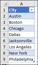
- In a new worksheet, type the entries you want to appear in your drop-down list. Ideally, you’ll have your list items in an Excel table. If you don’t, then you can quickly convert your list to a table by selecting any cell in the range, and pressing Ctrl+T.
- Why should you put your data in a table? When your data is in a table, then as you add or remove items from the list, any drop-downs you based on that table will automatically update. You don’t need to do anything else.
- Now is a good time to Sort data in a range or table in your drop-down list.
Note: If you can’t select Data Validation, the worksheet might be protected or shared. Unlock specific areas of a protected workbook or stop sharing the worksheet, and then try step 3 again.
- If you want a message to pop up when the cell is selected, check the Show input message when cell is selected box, and type a title and message in the boxes (up to 225 characters). If you don’t want a message to show up, clear the check box.
- If you want a message to pop up when someone enters something that’s not in your list, check the Show error alert after invalid data is entered box, pick an option from the Style box, and type a title and message. If you don’t want a message to show up, clear the check box.
- To show a message that doesn’t stop people from entering data that isn’t in the drop-down list, select Information or Warning. Information will show a message with this icon
 and Warning will show a message with this icon
  .
. - To stop people from entering data that isn’t in the drop-down list, select Stop.
Note: If you don’t add a title or text, the title defaults to «Microsoft Excel» and the message to: «The value you entered is not valid. A user has restricted values that can be entered into this cell.»
Working with your drop-down list
After you create your drop-down list, make sure it works the way you want. For example, you might want to check to see if Change the column width and row height to show all your entries.
If the list of entries for your drop-down list is on another worksheet and you want to prevent users from seeing it or making changes, consider hiding and protecting that worksheet. For more information about how to protect a worksheet, see Lock cells to protect them.
If you decide you want to change the options in your drop-down list, see Add or remove items from a drop-down list.
To delete a drop-down list, see Remove a drop-down list.
Create a drop-down list
You can help people work more efficiently in worksheets by using drop-down lists in cells. Drop-downs allow people to pick an item from a list that you create.
- In a new worksheet, type the entries you want to appear in your drop-down list. Ideally, you’ll have your list items in an Excel table. If you don’t, then you can quickly convert your list to a table by selecting any cell in the range, and pressing Ctrl+T.
- Why should you put your data in a table? When your data is in a table, then as you add or remove items from the list, any drop-downs you based on that table will automatically update. You don’t need to do anything else.
- Now is a good time to Sort data in a range or table in your drop-down list.
Note: If you can’t select Data Validation, the worksheet might be protected or shared. Unlock specific areas of a protected workbook or stop sharing the worksheet, and then try step 3 again.
- On the Settings tab, in the Allow box, select List.
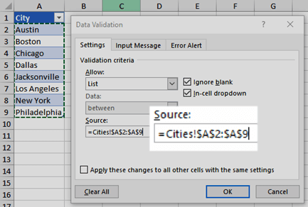
- Select in the Source box, then select your list range. We put ours on a sheet called Cities, in range A2:A9. Note that we left out the header row, because we don’t want that to be a selection option:
- If it’s OK for people to leave the cell empty, check the Ignore blank box.
- Check the In-cell dropdown box.
- Select the Input Message tab.
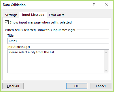
- If you want a message to pop up when the cell is selected, check the Show input message when cell is selected box, and type a title and message in the boxes (up to 225 characters). If you don’t want a message to show up, clear the check box.
- If you want a message to pop up when the cell is selected, check the Show input message when cell is selected box, and type a title and message in the boxes (up to 225 characters). If you don’t want a message to show up, clear the check box.
- Select the Error Alert tab.
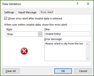
- If you want a message to pop up when someone enters something that’s not in your list, check the Show error alert after invalid data is entered box, pick an option from the Style box, and type a title and message. If you don’t want a message to show up, clear the check box.
- If you want a message to pop up when someone enters something that’s not in your list, check the Show error alert after invalid data is entered box, pick an option from the Style box, and type a title and message. If you don’t want a message to show up, clear the check box.
- Not sure which option to pick in the Style box?
- To show a message that doesn’t stop people from entering data that isn’t in the drop-down list, select Information or Warning. Information will show a message with this icon and Warning will show a message with this icon .
- To stop people from entering data that isn’t in the drop-down list, select Stop.
Note: If you don’t add a title or text, the title defaults to «Microsoft Excel» and the message to: «The value you entered is not valid. A user has restricted values that can be entered into this cell.»
Working with your drop-down list
After you create your drop-down list, make sure it works the way you want. For example, you might want to check to see if Change the column width and row height to show all your entries.
If the list of entries for your drop-down list is on another worksheet and you want to prevent users from seeing it or making changes, consider hiding and protecting that worksheet. For more information about how to protect a worksheet, see Lock cells to protect them.
If you decide you want to change the options in your drop-down list, see Add or remove items from a drop-down list.
To delete a drop-down list, see Remove a drop-down list.
How to make a dynamic dependent dropdown list in Excel an easy way

by Svetlana Cheusheva , updated on April 5, 2023
The tutorial shows how to create an Excel drop down list depending on another cell by using new dynamic array functions.
Creating a simple drop down list in Excel is easy. Making a multi-level cascading drop-down has always been a challenge. The above linked tutorial describes four different approaches, each including a crazy number of steps, a bunch of different formulas, and a handful of limitations relating to multi-word entries, blank cells, etc.
That was the bad news. The good news is that those methods were designed for pre-dynamic versions of Excel. The introduction of dynamic arrays in Excel 365 has changed everything! With new dynamic array functions, creating a multiple dependent drop-down list is a matter of minutes, if not seconds. No tricks, no caveats, no nonsense. Only fast, straightforward and easy-to-follow solutions.
- This new dynamic array way of making dropdown lists only works in Excel 365 and Excel 2021. In pre-dynamic Excel, you will have to do it the long old-fashioned way as described in Creating a dependent drop down in Excel 2019 — 2007.
- This solution is for a single row. If you want to copy your picklists down multiple rows, then follow the instructions in Dependent drop-down list for multiple rows.
How to make dynamic drop down list in Excel
This example demonstrates the general approach to creating a cascading drop down list in Excel by using the new dynamic array functions.
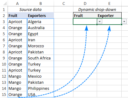
Supposing you have a list of fruit in column A and exporters in column B. An additional complication is that the fruit names are not grouped but scattered across the column. The goal is to put the unique fruit names in the first drop-down and depending on the user’s selection show the relevant exporters in the second drop-down.
To create a dynamic dependent drop down list in Excel, carry out these steps:
1. Get items for the main drop down list
For starters, we shall extract all different fruit names from column A. This can be done by using the UNIQUE function in its simplest form — supply the fruit list for the first argument (array) and omit the remaining optional arguments as their defaults work just fine for us:

The formula goes to G3, and after pressing the Enter key the results spill into the next cells automatically.
2. Create the main drop down
To make your primary drop-down list, configure an Excel Data Validation rule in this way:
- Select a cell in which you want the dropdown to appear (D3 in our case).
- On the Data tab, in the Data Tools group, click Data Validation.
- In the Data Validation dialog box, do the following:
- Under Allow, select List.
- In the Source box, enter the reference to the spill range output by the UNIQUE formula. For this, type the hash tag right after the cell reference, like this: =$G$3# This is called a spill range reference, and this syntax refers to the entire range regardless of how much it expands or contracts.
- Click OK to close the dialog.
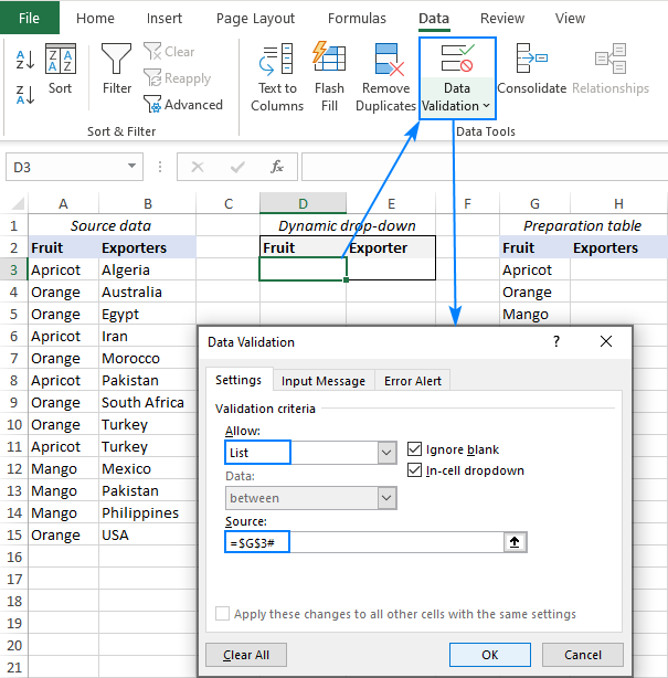

Your primary drop-down list is done!
3. Get items for the dependent drop down list
To get entries for the secondary dropdown menu, we’ll filter the values in column B based on the value selected in the first dropdown. This can be done with the help of another dynamic array function called FILTER:
Where B3:B15 are the source data for your dependent drop down, A3:A15 are the source data for your main dropdown, and D3 is the main dropdown cell.

To make sure the formula works correctly, you can select some value in the first drop-down list and observe the results returned by FILTER. Perfect! 🙂
4. Make the dependent drop down
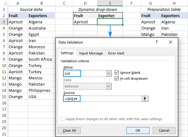
To create the second dropdown list, configure the data validation criteria exactly as you did for the first drop down at step 2. But this time, reference the spill range returned by the FILTER function: =$H$3#

That’s it! Your Excel dependent dropdown list is ready for use.
- To have the new entries included in the drop-down list automatically, format your source data as an Excel table. Or you can include a few blank cells in your formulas as demonstrated in this example.
- If your original data contains any gaps, you can filter out blanks by using this solution.
- To alphabetically sort a dropdown’s items, wrap your formulas in the SORT function as explained in this example.
How to create multiple dependent drop down list in Excel
In the previous example, we made a drop down list depending on another cell. But what if you need a multi-level hierarchy, i.e. a 3 rd dropdown depending in the 2 nd list, or even a 4 th dropdown depending on the 3 rd list. Is that possible? Yes, you can set up any number of dependent lists (a reasonable number, of course :).

For this example, we have placed states / provinces in column C, and are now looking to add a corresponding dropdown menu in G3:
To make a multiple dependent drop down list in Excel, this is what you need to do:
1. Set up the first drop down
The main dropdown list is created with exact the same steps as in the previous example (please see steps 1 and 2 above). The only difference is the spill range reference you enter in the Source box.

This time, the UNIQUE formula is in E8, and the main drop down list is going to be in E3. So, you select E3, click Data Validation, and supply this reference: =$E$8#
2. Configure the second drop down
As you may have noticed, now column B contains multiple occurrences of the same exporters. But you want only unique names in your dropdown list, right? To leave out all duplicate occurrences, wrap the UNIQUE function around your FILTER formula, and enter this updated formula in F8:
Where B3:B15 are the source data for the second drop down, A3:A15 are the source data for the first dropdown, and E3 is the first dropdown cell.
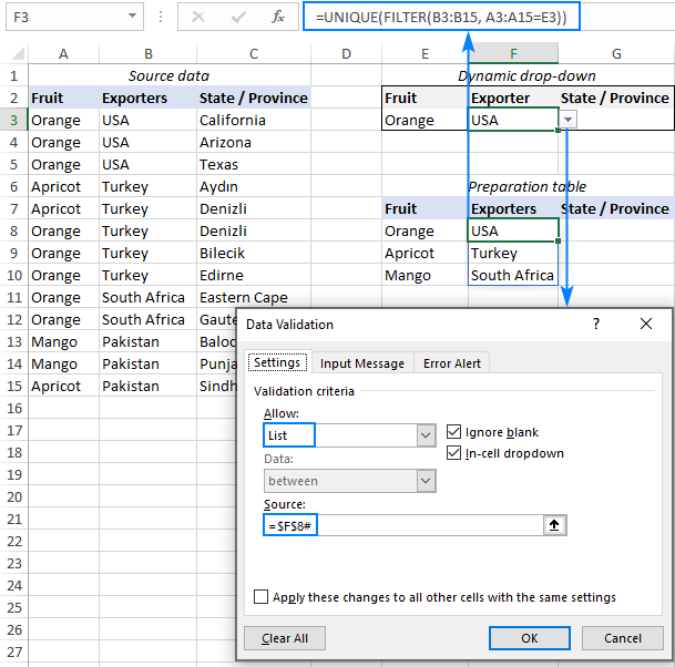
After that, use the following spill range reference for the Data Validation criteria: =$F$8#
3. Set up the third drop down
To gather the items for the 3 rd drop down list, make use of the FILTER formula with multiple criteria. The first criterion checks the entire fruit list against the value selected in the 1 st dropdown (A3:A15=E3) while the second criterion tests the list of exporters against the selection in the 2 nd dropdown (B3:B15=F3). The complete formula goes to G8:
=FILTER(C3:C15, (A3:A15=E3) * (B3:B15=F3))
If you are going to add more dependent dropdowns (4 th , 5 th , etc.), then most likely column C will contain multiple occurrences of the same item. To prevent duplicates from getting into the preparation table, and consequently in the 3rd dropdown, nest the FILTER formula in the UNIQUE function like we did in the previous step:
=UNIQUE(FILTER(C3:C15, (A3:A15=E3) * (B3:B15=F3)))

The last thing for you to do is to create one more Data Validation rule with this Source reference: =$G$8#
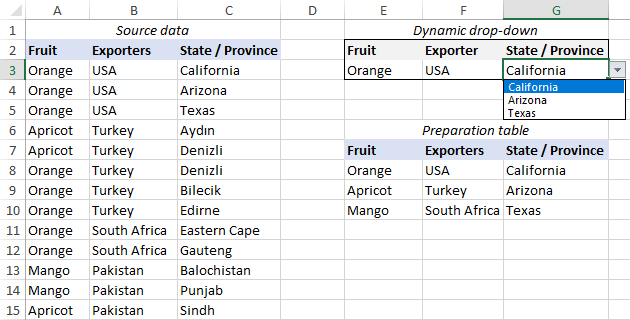
Your multiple dependent drop down list is good to go!
Tip. In a similar manner, you can get items for subsequent drop-downs. Assuming column D contains the source data for your 4 th dropdown list, you can enter the following formula in H8 to retrieve the corresponding items:
=UNIQUE(FILTER(D3:D15, (A3:A15=E3) * (B3:B15=F3) * (C3:C15=G3)))
How to make an expandable drop down list in Excel
After creating a dropdown, your first concern may be as to what happens when you add new items to the source data. Will the dropdown list update automatically? If your original data is formatted as Excel table, then yes, a dynamic drop down list discussed in the previous examples will expand automatically without any effort on your side because Excel tables are expandable by their nature.
If for some reason using an Excel table is not an option, you can make your dropdown list expandable in this way:
- To include new data automatically as it is added to the source list, add a few extra cells to the arrays referenced in your formulas.
- To exclude blank cells, configure the formulas to ignore empty cells until they get filled.
Keeping these two points in mind, let’s fine-tune the formulas in our data preparation table. The Data Validation rules do not require any adjustments at all.
Formula for the main dropdown
With the fruit names in A3:A15, we add 5 extra cells to the array to cater for possible new entries. Additionally, we embed the FILTER function into UNIQUE to extract unique values without blanks.
Given the above, the formula in G3 takes this shape:
Formula for the dependent dropdown
The formula in G3 does not need much tweaking — just extend the arrays with a few more cells:
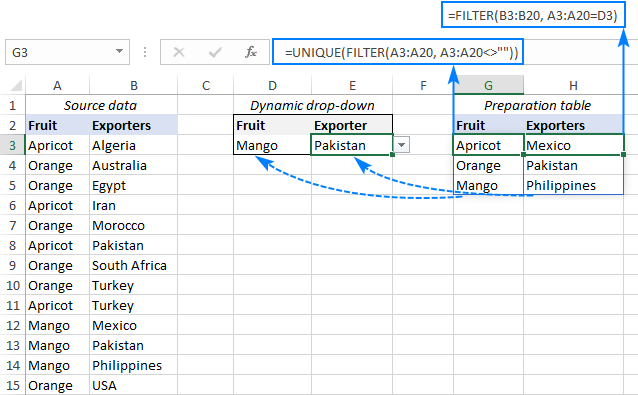
The result is a fully dynamic expandable dependent drop down list:
How to sort drop down list alphabetically
Want to arrange your dropdown list alphabetically without resorting the source data? The new dynamic Excel has a special function for this too! In your data preparation table, simply wrap the SORT function around your existing formulas.
The data validation rules are configured exactly as described in the previous examples.
To sort from A to Z
Since the ascending sort order is the default option, you can just nest your existing formulas in the array argument of SORT, omitting all other arguments which are optional.
For the main dropdown (the formula in G3):
For the dependent dropdown (the formula in H3):
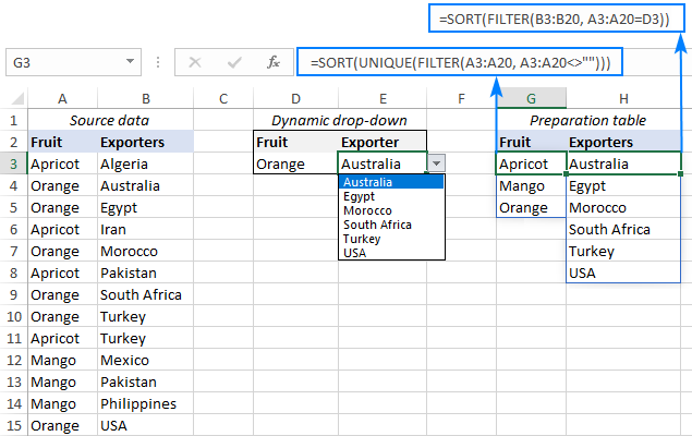
Done! Both drop down lists get sorted alphabetically A to Z.
To sort from Z to A
To sort in descending order, you need to set the 3 rd argument (sort_order) of the SORT function to -1.
For the main dropdown (the formula in G3):
=SORT(UNIQUE(FILTER(A3:A20, A3:A20<>«»)), 1, -1)
For the dependent dropdown (the formula in H3):
=SORT(FILTER(B3:B20, A3:A20=D3), 1, -1)
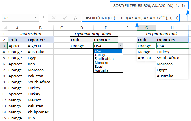
This will sort both the data in the preparation table and the items in the dropdown lists from Z to A:
Tip. Another fast and easy way to enter information in Excel spreadsheets is a data entry form.
That’s how to create dynamic drop down list in Excel with the help of the new dynamic array functions. Unlike the traditional methods, this approach works perfectly for single and multi-word entries and takes care of any blank cells. Thank you for reading and hope to see you on our blog next week!
Practice workbook for download
You may also be interested in
- Data validation in Excel with custom rules and formulas
- How to create dropdown list in Excel
- Create a multiple dependent drop down list in Excel 365 — 2010
- How to make multi-select drop down list in Excel
- How to make a drop down with images in Excel 365
- How to edit, copy and delete drop down list in Excel
5 способов сделать выпадающий список в ячейке Excel
Одной из наиболее полезных функций при вводе данных является возможность использовать выпадающий список в Excel. Он позволяет выбирать значение из предварительно определенного перечня и разрешает вводить только те данные, которые соответствуют вашим требованиям.
Мы предложим вам несколько простых способов, как сделать выпадающий список в Excel. Более сложные способы, основанные на динамических диапазонах и использовании данных из других таблиц, мы также рассмотрим.
Зачем нужен выпадающий список?
Часто случается так, что в какой-то из колонок вашей таблицы нужно вводить одинаковые повторяющиеся значения. К примеру, фамилии сотрудников, названия товаров или делать выбор в ячейке Excel вида «да – нет». Что может случиться? Конечно, в первую очередь будут ошибки при вводе. Человеческий фактор ведь никто не отменял. Чем нам сие грозит? К примеру, когда мы решим подсчитать, сколько заказов выполнил каждый из менеджеров, то окажется, что фамилий больше, чем сотрудников. Далее придётся искать ошибки, исправлять их и вновь повторять расчет.
Ну и конечно же, все время руками вводить одни и те же слова – просто бессмысленная работа и потеря времени. Вот здесь-то выпадающие списки нам и пригодятся. При нажатии выпадает перечень заранее определённых значений, из которых просто необходимо указать какое-то одно.
Важно то, что вы теперь будете не писать, а выбирать их с помощью мыши или клавиатуры. Это значительно ускоряет работу, а также гарантирует защиту от случайных ошибок. Проверка того, что мы записали в таблицу, теперь уже не нужна.
1 — Самый быстрый способ сделать выпадающий список.
Как проще всего добавить выпадающий список в таблицу Excel? Всего один щелчок правой кнопкой мыши по пустой клетке под столбцом с данными, затем команда контекстного меню «Выберите из раскрывающегося списка» (Choose from drop-down list). А можно просто стать в нужное место и нажать сочетание клавиш Alt+стрелка вниз . Появится отсортированный перечень уникальных ранее введенных значений.
Способ не работает, если нашу ячейку и столбец с записями отделяет хотя бы одна пустая строка или вы хотите ввести то, что еще не вводилось выше. На нашем примере это хорошо видно.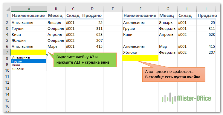
2 — Используем меню «Проверка данных» для создания выпадающего списка.
Давайте рассмотрим небольшой пример, в котором нам нужно постоянно вводить в таблицу одни и те же наименования товаров. Выпишите в столбик данные, которые мы будем использовать (например, названия товаров). В нашем примере — в диапазон G2:G7.
Выделите ячейку таблицы (можно сразу несколько), в которых хотите использовать ввод из заранее определенного перечня. Там мы разместим наш выпадающий список.
Далее в главном меню выберите на вкладке Данные – Проверка. (Data – Validation). Затем укажите пункт Тип данных (Allow) и выберите вариант Список (List). Поставьте курсор в поле Источник (Source) и впишите в него адреса с эталонными значениями элементов — в нашем случае G2:G7. Рекомендуется также использовать здесь абсолютные ссылки (для их установки нажмите клавишу F4).
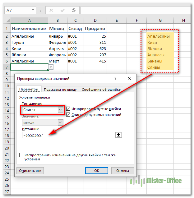
Бонусом здесь идет возможность задать подсказку и сообщение об ошибке, если автоматически вставленное значение вы захотите изменить вручную. Для этого существуют вкладки Подсказка по вводу (Input Message) и Сообщение об ошибке (Error Alert).
В качестве источника значений для выпадающего списка в Excel можно использовать также и именованный диапазон.
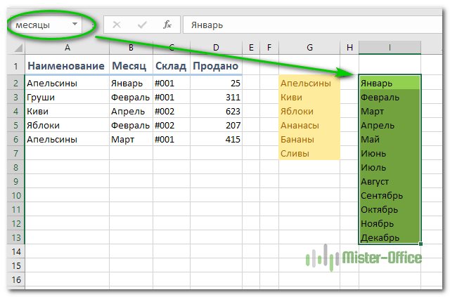
К примеру, диапазону I2:I13, содержащему названия месяцев, можно присвоить наименование «месяцы». Затем имя можно ввести в поле «Источник».
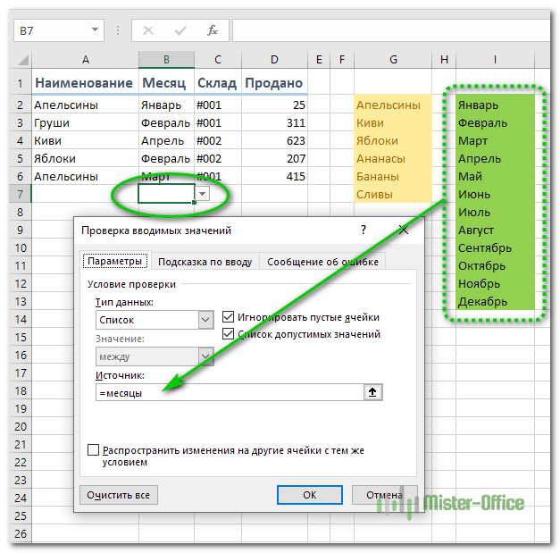
Кроме того, и источник и в виде обычного диапазона ячеек, и именованный диапазон могут находиться на других листах вашей рабочей книги.
Но вы можете и не использовать диапазоны или ссылки, а просто определить возможные варианты прямо в поле «Источник». К примеру, чтобы реализовать в таблице Excel простейший выбор «да – нет», вы можете вписать туда –
3 — Создаем элемент управления «Поле со списком».
Вставим на лист новый объект – элемент управления «Поле со списком» с последующей привязкой его к данным на листе Excel. Делаем:
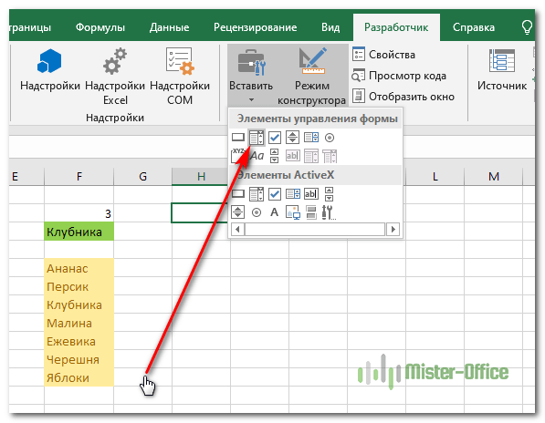
- Откройте вкладку Разработчик (Developer). Если её не видно, то в Excel 2007 нужно нажать кнопку Офис – Параметры – флажок Отображать вкладку Разработчик на ленте (Office Button – Options – Show Developer Tab in the Ribbon) или в версии 2010–2013 и выше щелкните правой кнопкой мыши по ленте, выберите команду Настройка ленты (Customize Ribbon) и включите отображение вкладки Разработчик (Developer) с помощью флажка.
- Найдите нужный значок среди элементов управления (см.рисунок ниже).
Вставив элемент управления на рабочий лист, щелкните по нему правой кнопкой мышки и выберите в появившемся меню пункт «Формат объекта». Далее указываем диапазон ячеек, в котором записаны допустимые значения для ввода. В поле «Связь с ячейкой» укажем, куда именно поместить результат. Важно учитывать, что этим результатом будет не само значение из указанного нами диапазона, а только его порядковый номер.
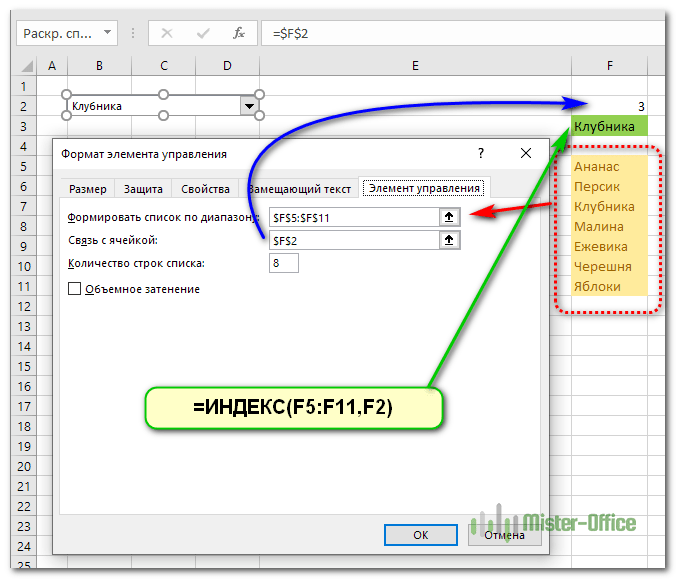
Но нам ведь нужен не этот номер, а соответствующее ему слово. Используем функцию ИНДЕКС (INDEX в английском варианте). Она позволяет найти в списке значений одно из них соответственно его порядковому номеру. В качестве аргументов ИНДЕКС укажите диапазон ячеек (F5:F11) и адрес с полученным порядковым номером (F2).
Формулу в F3 запишем, как показано на рисунке:
Как и в предыдущем способе, здесь возможны ссылки на другие листы, на именованные диапазоны.
Обратите также внимание, что здесь мы не привязаны ни к какой конкретному месту таблицы. Таким выпадающим списком Excel удобно пользоваться, поскольку его можно свободно «перетаскивать» мышкой в любое удобное место. Для этого на вкладке «Разработчик» нужно активизировать режим конструктора.
4 — Как сделать выпадающий список при помощи элемента ActiveX
Действуем аналогично предыдущему способу, но выбираем иконку чуть ниже — из раздела «Элементы ActiveX».
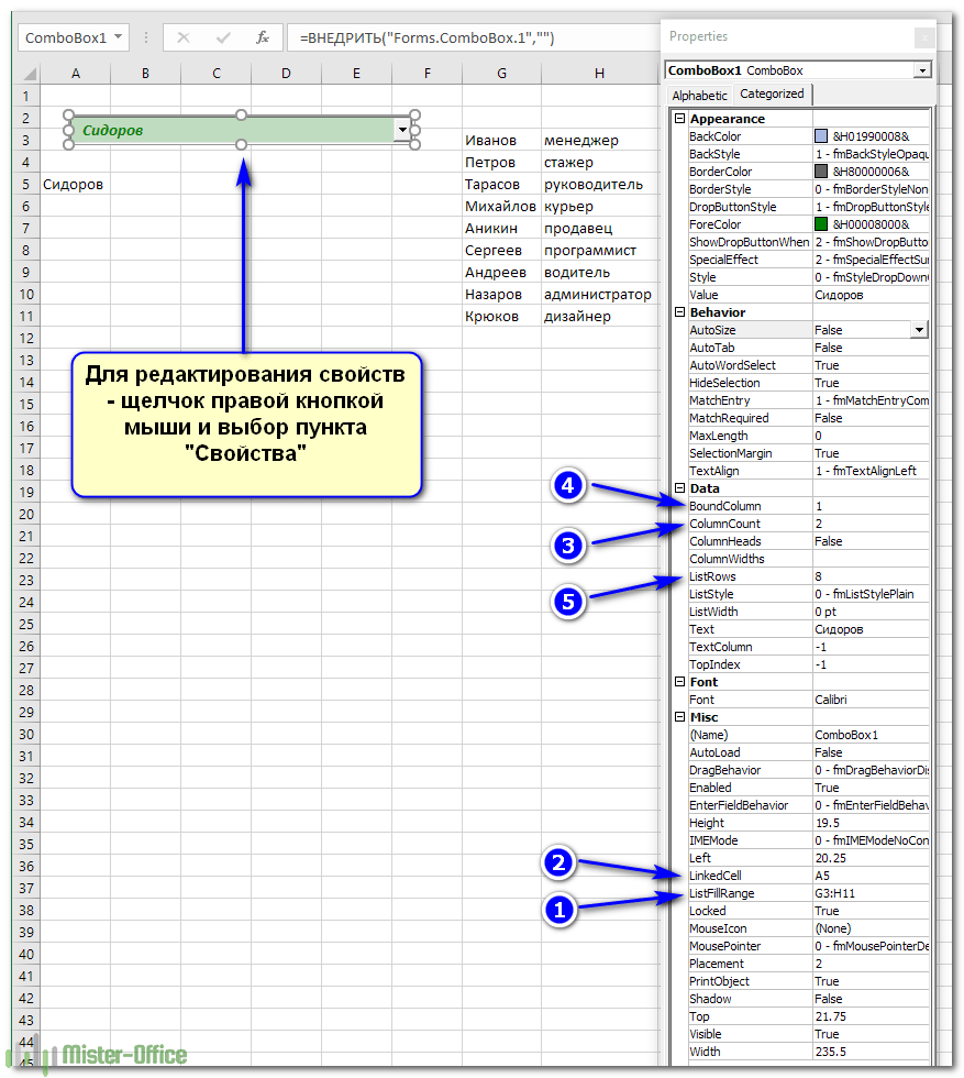
Определяем перечень допустимых значений (1). Обратите внимание, что здесь для показа можно выбирать сразу несколько колонок. Затем выбираем адрес, по которому будет вставлена нужная позиция из перечня (2).Указываем количество столбцов, которые будут использованы как исходные данные (3), и номер столбца, из которого будет происходить выбор для вставки на лист (4). Если укажете номер столбца 2, то в А5 будет вставлена не фамилия, а должность. Можно также указать количество строк, которое будет выведено в перечне. По умолчанию — 8. Остальные можно прокручивать мышкой (5).
Этот способ сложнее предыдущего, но зато возвращает сразу значение, а не его номер. Поэтому необходимость в промежуточной ячейке и обработке ее при помощи ИНДЕКС — отпадает. Думаю, таким выпадающим списком пользоваться гораздо удобнее.
5 — Как создать выпадающий список в Excel с автозаполнением
Задача: Сделать выпадающий список, в который будут автоматически добавляться значения из заданного динамического диапазона. Если в любую ячейку этого диапазона будут внесены изменения, то сразу изменится и набор предлагаемых к выбору значений. Никакие формулы и настройки здесь корректировать не нужно.
Вот как автозаполнение может выглядеть на простом примере:
Вариант 1. Укажите заведомо большой источник значений для списка.
Самая простая и несложная хитрость. В начале действуем по обычному алгоритму действий: в меню выбираем на вкладке Данные – Проверка . (Data – Validation). Из перечня Тип данных (Allow) выберите вариант Список (List). Поставьте курсор в поле Источник (Source). Зарезервируем в списке набор с большим запасом: например, до 55-й строки, хотя занято у нас только 7. Обязательно не забудьте поставить галочку в чекбоксе «Игнорировать пустые . «. Тогда ваш «резерв» из пустых значений не будет вам мешать.
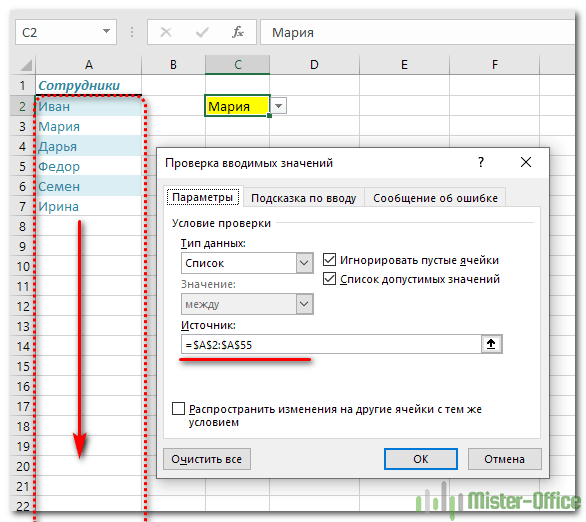
Действительно самый простой способ, но не слишком удобный. Ведь зарезервированное место может и закончиться.
Конечно, в качестве источника значений для выпадающего списка можно указать и весь столбец:
Но обработка такого большого количества ячеек может несколько замедлить вычисления. Особенно в больших таблицах Excel.
Вариант 2. Применяем именованный диапазон.
Именованный диапазон отличается от обычного тем, что ему присвоено определенное наименование. С ним гораздо проще работать, так как не нужно вводить ссылку, а достаточно просто указать его имя. Давайте рассмотрим небольшой пример.
В столбце А находятся имена сотрудников, которые мы будем вводить. Перечень может быть сколь угодно длинным. Нам необходимо, чтобы каждая новая запись включалась в раскрывающийся список без всяких дополнительных действий с нашей стороны.
Выделим имеющийся в нашем распоряжении перечень имен A2:A10. Затем присвоим ему название, заполнив поле «Имя», находящееся левее строки формул.
Так вы присвоите какое-то имя этому диапазону Excel.
Создадим в С2 перечень значений. В качестве источника для него укажем выражение
Недостатком работы с таким выпадающим списком в Excel является то, что новые значения нельзя просто дописывать в конец используемого перечня. Они останутся за пределами именованного диапазона. Если что-то нужно добавить, то их придется вставлять внутрь диапазона, использовав вставку пустой строки.
Перечень ещё можно отсортировать, чтобы удобно было пользоваться.
Главное неудобство пользования таким списком заключается в том, что используемый нами диапазон — статический. Автоматически его размеры измениться не могут. Согласитесь, не слишком удобный и технологичный способ. Слишком много ручных операций.
А теперь давайте пойдем дальше и посмотрим, как можно работать с динамическим диапазоном, который автоматически подстраивается под вводимые значения.
Вариант 3. Выпадающий список на основе «умной» таблицы Excel.
Начиная с 2007 года таблица для Excel — уже не просто набор строк и столбцов. Если вы просто расположите показатели с привычном для нас табличном виде, то он не будет считать их таблицей. Существует специальное форматирование, после чего диапазон начинает вести себя как единое целое, приобретая целый ряд интересных свойств. В частности, он начинает сам отслеживать свои размеры, динамически изменяясь при корректировке данных.
Любой набор значений в таблице может быть таким образом преобразован. Например, A1:A8. Выделите их мышкой. Затем преобразуйте в таблицу, используя меню Главная — Форматировать как таблицу (Home — Format as Table). Укажите, что в первой строке у вас находится название столбца. Это будет «шапка» вашей таблицы. Внешний вид может быть любым: это не более чем внешнее оформление и ни на что больше оно не влияет.
Как уже было сказано выше, «умная» таблица хороша для нас тем, что динамически меняет свои размеры при добавлении в нее информации. Если в строку ниже нее вписать что-либо, то она тут же присоединит к себе её. Таким образом, новые значения можно просто дописывать. К примеру, впишите в A9 слово «кокос», и таблица тут же расширится до 9 строк.
Следовательно, автоматическое обновление набора используемой информации в списке можно организовать, если использовать содержимое какого-либо столбца «умной» таблицы.
Осталось только обозначить ее как источник. Проблема заключается в том, что программа в качестве источника в списке не понимает выражение вида
и не считает его формулой. Хотя в обычных выражениях на листе вашей рабочей книги это вполне будет работать. Эта конструкция обозначает ссылку на первый столбец. Но в поле «Источник» она почему-то игнорируется.
Чтобы использовать «умную таблицу» как источник значений для выпадающего списка, нам придется пойти на небольшую хитрость и воспользоваться функцией ДВССЫЛ (INDIRECT в английском варианте). Эта функция преобразует текстовую переменную в обычную ссылку.
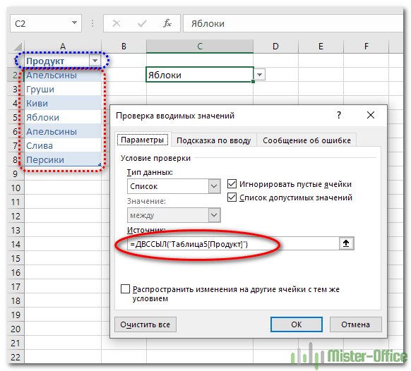
Формула теперь будет выглядеть следующим образом:
Таблица5 — имя, автоматически присвоенное «умной таблице». У вас оно может быть другим. На вкладке меню Конструктор (Design) можно изменить стандартное имя на свое (но без пробелов!). По нему мы сможем потом адресоваться к нашей таблице на любом листе книги.
Не забудьте также заключить все выражение в кавычки, чтобы обозначить его как текстовую переменную.
Теперь если в A9 вы допишете еще один фрукт (например, кокос), то он тут же автоматически появится и в нашем выпадающем списке. Аналогично будет, если мы что-то удалим. Задача автоматического увеличения выпадающего списка значений решена.
Надеемся, вы сможете теперь легко и быстро сделать выпадающий список в ячейке, чтобы с его помощью без ошибок вводить часто повторяющиеся данные в таблицу Excel.
- To show a message that doesn’t stop people from entering data that isn’t in the drop-down list, select Information or Warning. Information will show a message with this icon