Goal seek excel как использовать
На этом шаге мы рассмотрим параметры этого метода и пример применения .
Метод GoalSeek (Подбор параметра) подбирает значение параметра (неизвестной величины), являющееся решением уравнения с одной переменной. Предполагается, что уравнение приведено к виду: правая часть является постоянной, не зависящей от параметра, который входит только в левую часть уравнения. Вручную метод GoalSeek выполняется с помощью команды Сервис | Подбор параметра (Tools | Goal Seek) . Метод GoalSeek вычисляет корень, используя метод последовательных приближений, результат выполнения которого, вообще говоря, зависит от начального приближения. Поэтому для корректности нахождения корня надо позаботиться о корректном указании этого начального приближения.
Объект.GoalSeek(Goal, ChangingCell)
| Аргумент | Назначение |
|---|---|
| Объект | Ячейка, в которую введена формула, являющаяся правой частью решаемого уравнения. В этой формуле роль параметра (неизвестной величины) играет ссылка на ячейку, указанную в аргументе ChangingCell |
| Goal | Значение левой части решаемого уравнения, не содержащей параметра |
| ChangingCell | Ссылка на ячейку, отведенную под параметр (неизвестную величину). Значение, введенное в данную ячейку до активизации метода GoalSeek , рассматривается как начальное приближение к искомому корню |
Точность, с которой находится корень и предельно допустимое число итераций, используемых для нахождения корня, устанавливается свойствами MaxChange и MaxIterations объекта Application . Например, определение корня с точностью до 0,0001 максимум за 1000 итераций устанавливается инструкцией:
With Application .MaxIterations = 1000 .MaxChange = 0.0001 End With
Вручную эти величины устанавливаются на вкладке Вычисления (Calculation) диалогового окна Параметры (Options) , вызываемого командой Сервис | Параметры (Tools | Options) .
- Ячейку A1 отведем под неизвестную. Команда Подбор параметра (Goal Seek) находит корень уравнения методом последовательных приближений, результат которого зависит от начального приближения к корню. Команда Подбор параметра (Goal Seek) воспринимает значение, первоначально введенное в ячейку A1 , за начальное приближение. Будем считать, что начальное приближение к корню равно 0. Введем 0 в ячейку A1 . В методе GoalSeek аргумент ChangingCell отвечает за ссылку на ячейку, отведенную под неизвестную. В данном случае аргументу ChangingCell присваиваем Range («A1») .
- Ячейку А2 отведем под левую часть уравнения. При решении уравнения с помощью команды Подбор параметра (Goal Seek) уравнение надо преобразовать к такому виду, чтобы в правой его части содержалась только постоянная, не зависящая от неизвестной, которая должна входить только в его правую часть. В данном случае в ячейку А2 введем формулу =А1^2 (рисунок 1).
Рис.1. Ввод данных на рабочем листе при решении нелинейного уравнения
В методе GoalSeek диапазон, к которому применяется метод, отвечает за ссылку на ячейку, отведенную под левую часть уравнения, содержащую неизвестную. В данном случае метод GoalSeek применяется к диапазону Range («A2») .
Рис.2. Диалоговое окно Подбор параметра
- В поле Установить в ячейке (Set cell) введите ссылку на ячейку А2 ;
- В поле Изменяя значение ячейки (By changing cell) — ссылку на ячейку A1 ;
- В поле Значение введите 3. В поле Значение (То value) вводится величина правой части уравнения.
Range ("A2").GoalSeek Goal:=3, ChangingCell:=Range ("A1")
Рис.3. Результат выполнения команды
На следующем шаге мы рассмотрим метод Sort .
Use Goal Seek to find the result you want by adjusting an input value
If you know the result that you want from a formula, but are not sure what input value the formula needs to get that result, use the Goal Seek feature. For example, suppose that you need to borrow some money. You know how much money you want, how long you want to take to pay off the loan, and how much you can afford to pay each month. You can use Goal Seek to determine what interest rate you will need to secure in order to meet your loan goal.
If you know the result that you want from a formula, but are not sure what input value the formula needs to get that result, use the Goal Seek feature. For example, suppose that you need to borrow some money. You know how much money you want, how long you want to take to pay off the loan, and how much you can afford to pay each month. You can use Goal Seek to determine what interest rate you will need to secure in order to meet your loan goal.
Note: Goal Seek works only with one variable input value. If you want to accept more than one input value; for example, both the loan amount and the monthly payment amount for a loan, you use the Solver add-in. For more information, see Define and solve a problem by using Solver.
Step-by-step with an example
Let’s look at the preceding example, step-by-step.
Because you want to calculate the loan interest rate needed to meet your goal, you use the PMT function. The PMT function calculates a monthly payment amount. In this example, the monthly payment amount is the goal that you seek.
Prepare the worksheet
- Open a new, blank worksheet.
- First, add some labels in the first column to make it easier to read the worksheet.
- In cell A1, type Loan Amount.
- In cell A2, type Term in Months.
- In cell A3, type Interest Rate.
- In cell A4, type Payment.
Note: Although you know the payment amount that you want, you do not enter it as a value, because the payment amount is a result of the formula. Instead, you add the formula to the worksheet and specify the payment value at a later step, when you use Goal Seek.
- In cell B4, type =PMT(B3/12,B2,B1). This formula calculates the payment amount. In this example, you want to pay $900 each month. You don’t enter that amount here, because you want to use Goal Seek to determine the interest rate, and Goal Seek requires that you start with a formula. The formula refers to cells B1 and B2, which contain values that you specified in preceding steps. The formula also refers to cell B3, which is where you will specify that Goal Seek put the interest rate. The formula divides the value in B3 by 12 because you specified a monthly payment, and the PMT function assumes an annual interest rate. Because there is no value in cell B3, Excel assumes a 0% interest rate and, using the values in the example, returns a payment of $555.56. You can ignore that value for now.
Use Goal Seek to determine the interest rate
- On the Data tab, in the Data Tools group, click What-If Analysis, and then click Goal Seek.
- In the Set cell box, enter the reference for the cell that contains the formula that you want to resolve. In the example, this reference is cell B4.
- In the To value box, type the formula result that you want. In the example, this is -900. Note that this number is negative because it represents a payment.
- In the By changing cell box, enter the reference for the cell that contains the value that you want to adjust. In the example, this reference is cell B3.
Note: The cell that Goal Seek changes must be referenced by the formula in the cell that you specified in the Set cell box.
Goal Seek runs and produces a result, as shown in the following illustration.
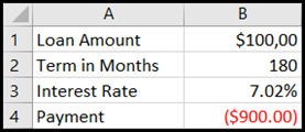
Cells B1, B2, and B3 are the values for the loan amount, term length, and interest rate. Cell B4 displays the result of the formula =PMT(B3/12,B2,B1).
- Finally, format the target cell (B3) so that it displays the result as a percentage.
- On the Home tab, in the Number group, click Percentage.
- Click Increase Decimal or Decrease Decimal to set the number of decimal places.
If you know the result that you want from a formula, but are not sure what input value the formula needs to get that result, use the Goal Seek feature. For example, suppose that you need to borrow some money. You know how much money you want, how long you want to take to pay off the loan, and how much you can afford to pay each month. You can use Goal Seek to determine what interest rate you will need to secure in order to meet your loan goal.
Note: Goal Seek works only with one variable input value. If you want to accept more than one input value, for example, both the loan amount and the monthly payment amount for a loan, use the Solver add-in. For more information, see Define and solve a problem by using Solver.
Step-by-step with an example
Let’s look at the preceding example, step-by-step.
Because you want to calculate the loan interest rate needed to meet your goal, you use the PMT function. The PMT function calculates a monthly payment amount. In this example, the monthly payment amount is the goal that you seek.
Prepare the worksheet
- Open a new, blank worksheet.
- First, add some labels in the first column to make it easier to read the worksheet.
- In cell A1, type Loan Amount.
- In cell A2, type Term in Months.
- In cell A3, type Interest Rate.
- In cell A4, type Payment.
Note: Although you know the payment amount that you want, you do not enter it as a value, because the payment amount is a result of the formula. Instead, you add the formula to the worksheet and specify the payment value at a later step, when you use Goal Seek.
- In cell B4, type =PMT(B3/12,B2,B1). This formula calculates the payment amount. In this example, you want to pay $900 each month. You don’t enter that amount here, because you want to use Goal Seek to determine the interest rate, and Goal Seek requires that you start with a formula. The formula refers to cells B1 and B2, which contain values that you specified in preceding steps. The formula also refers to cell B3, which is where you will specify that Goal Seek put the interest rate. The formula divides the value in B3 by 12 because you specified a monthly payment, and the PMT function assumes an annual interest rate. Because there is no value in cell B3, Excel assumes a 0% interest rate and, using the values in the example, returns a payment of $555.56. You can ignore that value for now.
Use Goal Seek to determine the interest rate
- Do one of the following: In Excel 2016 for Mac: On the Data tab, click What-If Analysis, and then click Goal Seek. In Excel for Mac 2011: On the Data tab, in the Data Tools group, click What-If Analysis, and then click Goal Seek.
- In the Set cell box, enter the reference for the cell that contains the formula that you want to resolve. In the example, this reference is cell B4.
- In the To value box, type the formula result that you want. In the example, this is -900. Note that this number is negative because it represents a payment.
- In the By changing cell box, enter the reference for the cell that contains the value that you want to adjust. In the example, this reference is cell B3.
Note: The cell that Goal Seek changes must be referenced by the formula in the cell that you specified in the Set cell box.
Goal Seek runs and produces a result, as shown in the following illustration.
- Finally, format the target cell (B3) so that it displays the result as a percentage. Follow one of these steps:
- In Excel 2016 for Mac: On the Home tab, click Increase Decimal
 or Decrease Decimal
 .
. - In Excel for Mac 2011: On the Home tab, under Number group, click Increase Decimal or Decrease Decimal to set the number of decimal places.
- In Excel 2016 for Mac: On the Home tab, click Increase Decimal
Use Goal Seek to find the result you want by adjusting an input value
If you know the result that you want from a formula, but are not sure what input value the formula needs to get that result, use the Goal Seek feature. For example, suppose that you need to borrow some money. You know how much money you want, how long you want to take to pay off the loan, and how much you can afford to pay each month. You can use Goal Seek to determine what interest rate you will need to secure in order to meet your loan goal.
If you know the result that you want from a formula, but are not sure what input value the formula needs to get that result, use the Goal Seek feature. For example, suppose that you need to borrow some money. You know how much money you want, how long you want to take to pay off the loan, and how much you can afford to pay each month. You can use Goal Seek to determine what interest rate you will need to secure in order to meet your loan goal.
Note: Goal Seek works only with one variable input value. If you want to accept more than one input value; for example, both the loan amount and the monthly payment amount for a loan, you use the Solver add-in. For more information, see Define and solve a problem by using Solver.
Step-by-step with an example
Let’s look at the preceding example, step-by-step.
Because you want to calculate the loan interest rate needed to meet your goal, you use the PMT function. The PMT function calculates a monthly payment amount. In this example, the monthly payment amount is the goal that you seek.
Prepare the worksheet
- Open a new, blank worksheet.
- First, add some labels in the first column to make it easier to read the worksheet.
- In cell A1, type Loan Amount.
- In cell A2, type Term in Months.
- In cell A3, type Interest Rate.
- In cell A4, type Payment.
Note: Although you know the payment amount that you want, you do not enter it as a value, because the payment amount is a result of the formula. Instead, you add the formula to the worksheet and specify the payment value at a later step, when you use Goal Seek.
- In cell B4, type =PMT(B3/12,B2,B1). This formula calculates the payment amount. In this example, you want to pay $900 each month. You don’t enter that amount here, because you want to use Goal Seek to determine the interest rate, and Goal Seek requires that you start with a formula. The formula refers to cells B1 and B2, which contain values that you specified in preceding steps. The formula also refers to cell B3, which is where you will specify that Goal Seek put the interest rate. The formula divides the value in B3 by 12 because you specified a monthly payment, and the PMT function assumes an annual interest rate. Because there is no value in cell B3, Excel assumes a 0% interest rate and, using the values in the example, returns a payment of $555.56. You can ignore that value for now.
Use Goal Seek to determine the interest rate
- On the Data tab, in the Data Tools group, click What-If Analysis, and then click Goal Seek.
- In the Set cell box, enter the reference for the cell that contains the formula that you want to resolve. In the example, this reference is cell B4.
- In the To value box, type the formula result that you want. In the example, this is -900. Note that this number is negative because it represents a payment.
- In the By changing cell box, enter the reference for the cell that contains the value that you want to adjust. In the example, this reference is cell B3.
Note: The cell that Goal Seek changes must be referenced by the formula in the cell that you specified in the Set cell box.
Goal Seek runs and produces a result, as shown in the following illustration.
Cells B1, B2, and B3 are the values for the loan amount, term length, and interest rate. Cell B4 displays the result of the formula =PMT(B3/12,B2,B1).
- Finally, format the target cell (B3) so that it displays the result as a percentage.
- On the Home tab, in the Number group, click Percentage.
- Click Increase Decimal or Decrease Decimal to set the number of decimal places.
If you know the result that you want from a formula, but are not sure what input value the formula needs to get that result, use the Goal Seek feature. For example, suppose that you need to borrow some money. You know how much money you want, how long you want to take to pay off the loan, and how much you can afford to pay each month. You can use Goal Seek to determine what interest rate you will need to secure in order to meet your loan goal.
Note: Goal Seek works only with one variable input value. If you want to accept more than one input value, for example, both the loan amount and the monthly payment amount for a loan, use the Solver add-in. For more information, see Define and solve a problem by using Solver.
Step-by-step with an example
Let’s look at the preceding example, step-by-step.
Because you want to calculate the loan interest rate needed to meet your goal, you use the PMT function. The PMT function calculates a monthly payment amount. In this example, the monthly payment amount is the goal that you seek.
Prepare the worksheet
- Open a new, blank worksheet.
- First, add some labels in the first column to make it easier to read the worksheet.
- In cell A1, type Loan Amount.
- In cell A2, type Term in Months.
- In cell A3, type Interest Rate.
- In cell A4, type Payment.
Note: Although you know the payment amount that you want, you do not enter it as a value, because the payment amount is a result of the formula. Instead, you add the formula to the worksheet and specify the payment value at a later step, when you use Goal Seek.
- In cell B4, type =PMT(B3/12,B2,B1). This formula calculates the payment amount. In this example, you want to pay $900 each month. You don’t enter that amount here, because you want to use Goal Seek to determine the interest rate, and Goal Seek requires that you start with a formula. The formula refers to cells B1 and B2, which contain values that you specified in preceding steps. The formula also refers to cell B3, which is where you will specify that Goal Seek put the interest rate. The formula divides the value in B3 by 12 because you specified a monthly payment, and the PMT function assumes an annual interest rate. Because there is no value in cell B3, Excel assumes a 0% interest rate and, using the values in the example, returns a payment of $555.56. You can ignore that value for now.
Use Goal Seek to determine the interest rate
- Do one of the following: In Excel 2016 for Mac: On the Data tab, click What-If Analysis, and then click Goal Seek. In Excel for Mac 2011: On the Data tab, in the Data Tools group, click What-If Analysis, and then click Goal Seek.
- In the Set cell box, enter the reference for the cell that contains the formula that you want to resolve. In the example, this reference is cell B4.
- In the To value box, type the formula result that you want. In the example, this is -900. Note that this number is negative because it represents a payment.
- In the By changing cell box, enter the reference for the cell that contains the value that you want to adjust. In the example, this reference is cell B3.
Note: The cell that Goal Seek changes must be referenced by the formula in the cell that you specified in the Set cell box.
Goal Seek runs and produces a result, as shown in the following illustration.
- Finally, format the target cell (B3) so that it displays the result as a percentage. Follow one of these steps:
- In Excel 2016 for Mac: On the Home tab, click Increase Decimalor Decrease Decimal.
- In Excel for Mac 2011: On the Home tab, under Number group, click Increase Decimal or Decrease Decimal to set the number of decimal places.
- In Excel 2016 for Mac: On the Home tab, click Increase Decimal
Use Goal Seek to find the result you want by adjusting an input value
If you know the result that you want from a formula, but are not sure what input value the formula needs to get that result, use the Goal Seek feature. For example, suppose that you need to borrow some money. You know how much money you want, how long you want to take to pay off the loan, and how much you can afford to pay each month. You can use Goal Seek to determine what interest rate you will need to secure in order to meet your loan goal.
If you know the result that you want from a formula, but are not sure what input value the formula needs to get that result, use the Goal Seek feature. For example, suppose that you need to borrow some money. You know how much money you want, how long you want to take to pay off the loan, and how much you can afford to pay each month. You can use Goal Seek to determine what interest rate you will need to secure in order to meet your loan goal.
Note: Goal Seek works only with one variable input value. If you want to accept more than one input value; for example, both the loan amount and the monthly payment amount for a loan, you use the Solver add-in. For more information, see Define and solve a problem by using Solver.
Step-by-step with an example
Let’s look at the preceding example, step-by-step.
Because you want to calculate the loan interest rate needed to meet your goal, you use the PMT function. The PMT function calculates a monthly payment amount. In this example, the monthly payment amount is the goal that you seek.
Prepare the worksheet
- Open a new, blank worksheet.
- First, add some labels in the first column to make it easier to read the worksheet.
- In cell A1, type Loan Amount.
- In cell A2, type Term in Months.
- In cell A3, type Interest Rate.
- In cell A4, type Payment.
Note: Although you know the payment amount that you want, you do not enter it as a value, because the payment amount is a result of the formula. Instead, you add the formula to the worksheet and specify the payment value at a later step, when you use Goal Seek.
- In cell B4, type =PMT(B3/12,B2,B1). This formula calculates the payment amount. In this example, you want to pay $900 each month. You don’t enter that amount here, because you want to use Goal Seek to determine the interest rate, and Goal Seek requires that you start with a formula. The formula refers to cells B1 and B2, which contain values that you specified in preceding steps. The formula also refers to cell B3, which is where you will specify that Goal Seek put the interest rate. The formula divides the value in B3 by 12 because you specified a monthly payment, and the PMT function assumes an annual interest rate. Because there is no value in cell B3, Excel assumes a 0% interest rate and, using the values in the example, returns a payment of $555.56. You can ignore that value for now.
Use Goal Seek to determine the interest rate
- On the Data tab, in the Data Tools group, click What-If Analysis, and then click Goal Seek.
- In the Set cell box, enter the reference for the cell that contains the formula that you want to resolve. In the example, this reference is cell B4.
- In the To value box, type the formula result that you want. In the example, this is -900. Note that this number is negative because it represents a payment.
- In the By changing cell box, enter the reference for the cell that contains the value that you want to adjust. In the example, this reference is cell B3.
Note: The cell that Goal Seek changes must be referenced by the formula in the cell that you specified in the Set cell box.
Goal Seek runs and produces a result, as shown in the following illustration.
Cells B1, B2, and B3 are the values for the loan amount, term length, and interest rate. Cell B4 displays the result of the formula =PMT(B3/12,B2,B1).
- Finally, format the target cell (B3) so that it displays the result as a percentage.
- On the Home tab, in the Number group, click Percentage.
- Click Increase Decimal or Decrease Decimal to set the number of decimal places.
If you know the result that you want from a formula, but are not sure what input value the formula needs to get that result, use the Goal Seek feature. For example, suppose that you need to borrow some money. You know how much money you want, how long you want to take to pay off the loan, and how much you can afford to pay each month. You can use Goal Seek to determine what interest rate you will need to secure in order to meet your loan goal.
Note: Goal Seek works only with one variable input value. If you want to accept more than one input value, for example, both the loan amount and the monthly payment amount for a loan, use the Solver add-in. For more information, see Define and solve a problem by using Solver.
Step-by-step with an example
Let’s look at the preceding example, step-by-step.
Because you want to calculate the loan interest rate needed to meet your goal, you use the PMT function. The PMT function calculates a monthly payment amount. In this example, the monthly payment amount is the goal that you seek.
Prepare the worksheet
- Open a new, blank worksheet.
- First, add some labels in the first column to make it easier to read the worksheet.
- In cell A1, type Loan Amount.
- In cell A2, type Term in Months.
- In cell A3, type Interest Rate.
- In cell A4, type Payment.
Note: Although you know the payment amount that you want, you do not enter it as a value, because the payment amount is a result of the formula. Instead, you add the formula to the worksheet and specify the payment value at a later step, when you use Goal Seek.
- In cell B4, type =PMT(B3/12,B2,B1). This formula calculates the payment amount. In this example, you want to pay $900 each month. You don’t enter that amount here, because you want to use Goal Seek to determine the interest rate, and Goal Seek requires that you start with a formula. The formula refers to cells B1 and B2, which contain values that you specified in preceding steps. The formula also refers to cell B3, which is where you will specify that Goal Seek put the interest rate. The formula divides the value in B3 by 12 because you specified a monthly payment, and the PMT function assumes an annual interest rate. Because there is no value in cell B3, Excel assumes a 0% interest rate and, using the values in the example, returns a payment of $555.56. You can ignore that value for now.
Use Goal Seek to determine the interest rate
- Do one of the following: In Excel 2016 for Mac: On the Data tab, click What-If Analysis, and then click Goal Seek. In Excel for Mac 2011: On the Data tab, in the Data Tools group, click What-If Analysis, and then click Goal Seek.
- In the Set cell box, enter the reference for the cell that contains the formula that you want to resolve. In the example, this reference is cell B4.
- In the To value box, type the formula result that you want. In the example, this is -900. Note that this number is negative because it represents a payment.
- In the By changing cell box, enter the reference for the cell that contains the value that you want to adjust. In the example, this reference is cell B3.
Note: The cell that Goal Seek changes must be referenced by the formula in the cell that you specified in the Set cell box.
Goal Seek runs and produces a result, as shown in the following illustration.
- Finally, format the target cell (B3) so that it displays the result as a percentage. Follow one of these steps:
- In Excel 2016 for Mac: On the Home tab, click Increase Decimalor Decrease Decimal.
- In Excel for Mac 2011: On the Home tab, under Number group, click Increase Decimal or Decrease Decimal to set the number of decimal places.
- In Excel 2016 for Mac: On the Home tab, click Increase Decimal