Как считать проценты в гугл таблице
Join us and leaders from Brex, Carta, and others for a B2B SaaS Pricing Webinar on Nov 8th! Save your spot.

We raised a $20m Series A led by Coatue + Accel! Click here to read the announcement.
We’re live on Product Hunt and would love your support! Join the discussion.
Google Sheets
How to Calculate Percentage in Google Sheets

Google Sheets, a cloud-based spreadsheet program, is a versatile tool that can be used for a variety of tasks. One such task is calculating percentages, a fundamental concept in many fields such as business, finance, and education. Understanding how to calculate percentages in Google Sheets can help you analyze data and make informed decisions. This guide will walk you through the process, step by step.
Understanding the Concept of Percentage
Before diving into the technicalities of , it’s important to understand what a percentage is. Essentially, a percentage is a way of expressing a number as a fraction of 100. It is often used to compare the size of a part to the whole. For example, if you score 90 out of 100 in a test, your score can be expressed as 90%.
Percentages are used in a wide range of applications, from calculating discounts and interest rates to analyzing survey results and statistical data. Knowing how to calculate percentages is a valuable skill in many areas of life.
Basic Formula for Calculating Percentage
In Google Sheets, the basic formula for calculating percentage is as follows: (Part/Whole)*100. This formula divides the part by the whole and then multiplies the result by 100 to get the percentage. For example, if you want to find out what percentage 50 is of 200, you would divide 50 by 200 and then multiply the result by 100. The result would be 25%.
It’s important to note that Google Sheets automatically formats the result as a percentage. This means that if your result is 0.25, Google Sheets will display it as 25%. If you want to see the decimal result, you can change the format of the cell to ‘Number’.
Using Google Sheets to Calculate Percentage
Step-by-Step Guide
Now that you understand the basic concept and formula for calculating percentages, let’s look at how to do this in Google Sheets. Here’s a step-by-step guide:
- Open a new Google Sheets document.
- In cell A1, enter the whole number. In cell B1, enter the part number.
- In cell C1, enter the formula: =(B1/A1)*100
- Press ‘Enter’. The result will be displayed in cell C1.
This is the simplest way to calculate percentages in Google Sheets. However, there are also more complex calculations you can perform, depending on your needs.
Calculating Percentage Increase or Decrease
If you want to calculate the percentage increase or decrease between two numbers, you can use the following formula: ((New Number — Old Number)/Old Number)*100. This formula subtracts the old number from the new number, divides the result by the old number, and then multiplies by 100 to get the percentage.
For example, if a product’s price increased from $100 to $120, the percentage increase would be ((120-100)/100)*100, which equals 20%.
Calculating Percentage of a Total
If you have a list of numbers and you want to find out what percentage each number is of the total, you can use the SUM function in combination with the basic percentage formula. Here’s how:
- Enter your list of numbers in column A.
- In cell B1, enter the formula: =SUM(A:A). This will calculate the total of all numbers in column A.
- In cell C1, enter the formula: =(A1/B1)*100. This will calculate what percentage the number in cell A1 is of the total.
- Drag the fill handle (the small square in the bottom-right corner of the cell) down to copy the formula to the rest of the cells in column C.
The result will be a column of percentages, each representing what portion of the total the corresponding number in column A is.
Conclusion
Calculating percentages in Google Sheets is a straightforward process once you understand the basic formula and how to apply it. Whether you’re calculating a simple percentage, a percentage increase or decrease, or the percentage of a total, Google Sheets provides the tools you need to perform these calculations with ease. With this guide, you should now be able to calculate percentages in Google Sheets like a pro.
Take Your Percentage Calculations Further with Causal
Now that you’re equipped to handle percentages in Google Sheets, imagine taking your data analysis to the next level. Causal is designed specifically for numerical data and calculations, offering a powerful alternative to traditional spreadsheets. With its intuitive modelling, forecasting, and scenario planning capabilities, plus stunning data visualizations and interactive dashboards, Causal streamlines your workflow and enhances your decision-making process. Ready to elevate your data game? Sign up today and experience the simplicity and efficiency of Causal for free.
Как сделать динамическую шкалу выполнения задач в Google Таблицах
Ведение записей о достижении определенных целей – один из возможных сценариев использования Google Таблиц. Вы можете указывать задачи в процентах и выводить их общий статус выполнения. Для наглядности можно реализовать графическую шкалу с разными цветами, что я и предлагаю сделать в рамках этой статьи.
Исходные материалы
Скорее всего, наполнение таблицы, которую я взял в качестве исходника, значительно будет отличаться от той, что имеется у вас в наличии. Поэтому я постарался сделать максимально отстраненную от какой-либо темы общую таблицу, поместив в нее основные материалы.
- Соответственно, понадобится определенное количество пунктов, для которых вы можете указывать проценты выполнения. Сами проценты вписываются вручную или выбираются из выпадающего списка, о создании которого я уже рассказывал в другой статье.
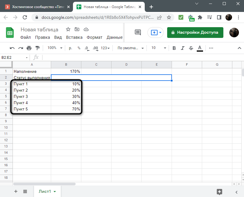
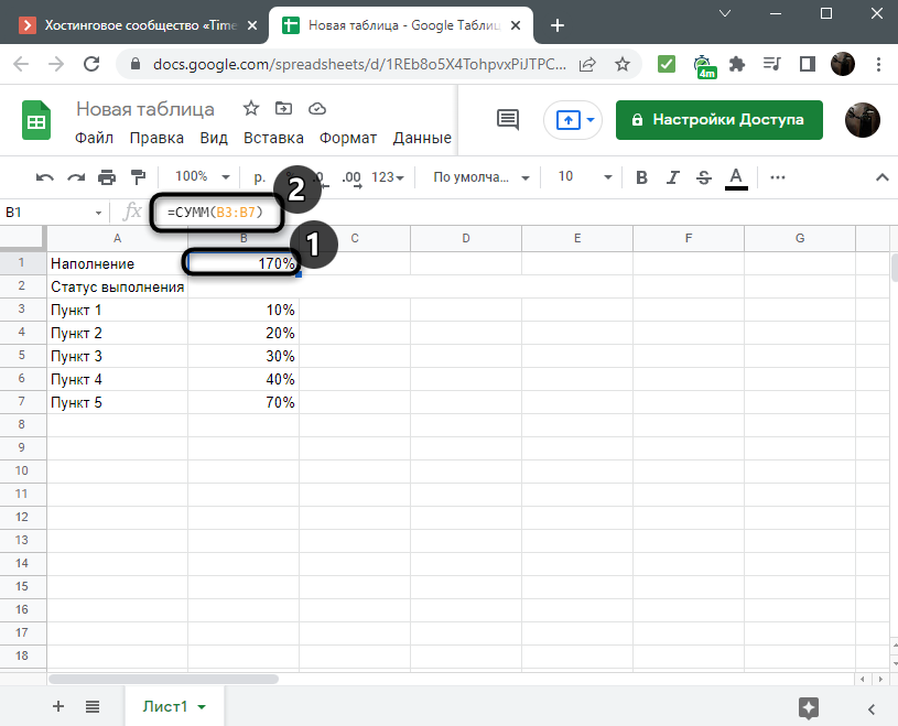
- Далее – свободная ячейка, в которой будет отображаться общее значение в процентах. Вам требуется простая формула суммирования. Формат ячейки обязательно должен быть в процентах, чтобы значение соответствовало всем остальным в таблице.
- Теперь самое главное – место для создания графической шкалы. На следующем скриншоте вы видите, что для нее я объединил несколько последовательных ячеек слева и дал название этой демонстрации.
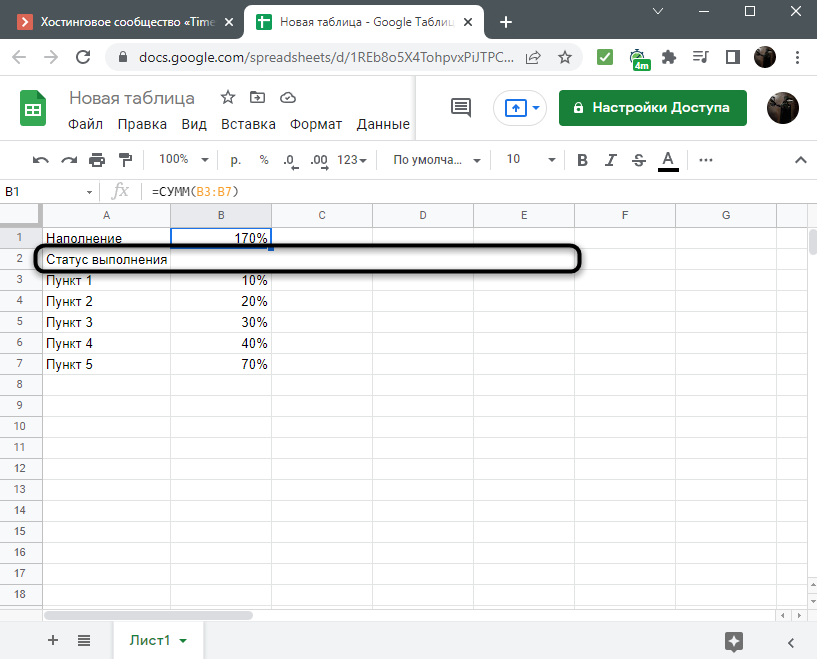
Быстро пробежимся по последнему пункту более детально, чтобы разобраться с тем, как объединить несколько ячеек в одну, если ранее вы не сталкивались с подобной задачей.
- Сначала выделите горизонтальную последовательность ячеек и откройте меню «Формат».
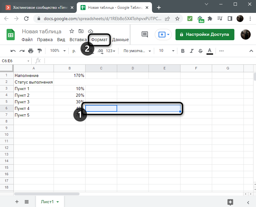
- Наведите курсор на пункт «Объединить ячейки» и выберите вариант «Объединить все».
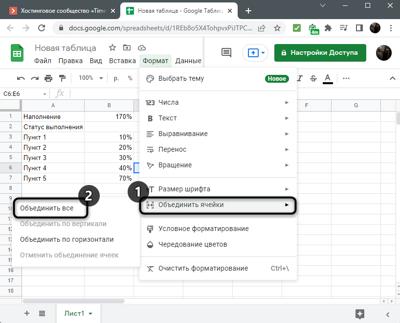
- Вернитесь к таблице и убедитесь в том, что настройка выполнена успешно.
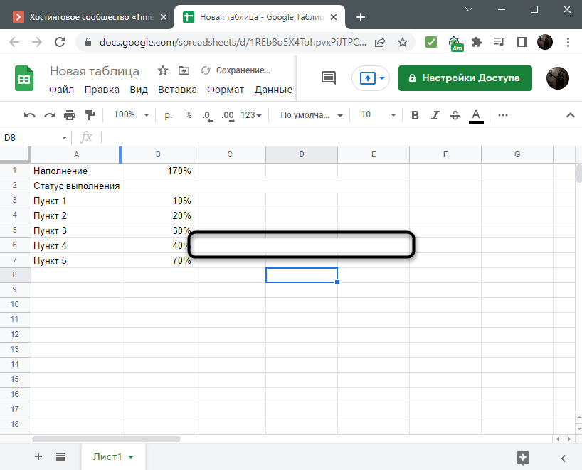
На этом подготовительные работы можно считать завершенными. Теперь вы понимаете, что показано на скриншотах в моих инструкциях и сможете реализовать создание сложной формулы (о которой пойдет речь далее), изменив ее значения под имеющиеся в таблице данные.
Комьюнити теперь в Телеграм
Подпишитесь и будьте в курсе последних IT-новостей
Создание графической шкалы выполнения задач
Функция SPARKLINE представляет собой миниатюрную диаграмму, расположенную внутри одной ячейки. Мы объединили несколько ячеек в одну, поэтому диаграмма будет растягиваться. Понадобится только выбрать правильный тип и установить, что именно она будет считать. Все это осуществляется при помощи небольшой формулы:
- Выберите ту самую объединенную ячейку, объявите функцию =SPARKLINE(), внутри скобок укажите номер ячейки, в которой отображается сумма всех процентов. Соответственно, не забудьте поставить точку с запятой.
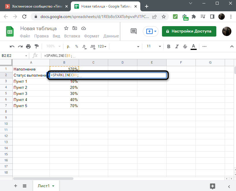
- Заполните остальную часть функции, которая выглядит так: . О каждом из этих параметров более детально поговорим ниже. Номера ячеек для подсчета замените на свои (указывайте ячейки не с процентами, а с названиями пунктов, что видно на следующем изображении).
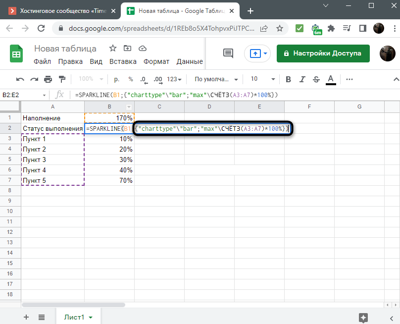
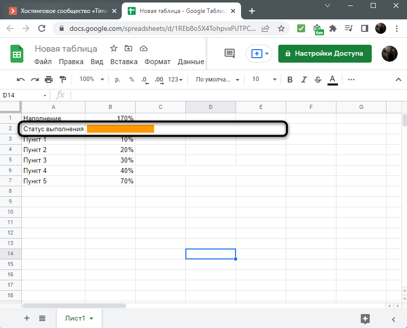
- Нажмите Enter для применения изменений и посмотрите, появилась ли на экране графическая шкала. Если нет, скорее всего, у вас еще не указаны проценты в соответствующих полях. В противном случае внимательно проверьте то, как именно вы написали формулу.
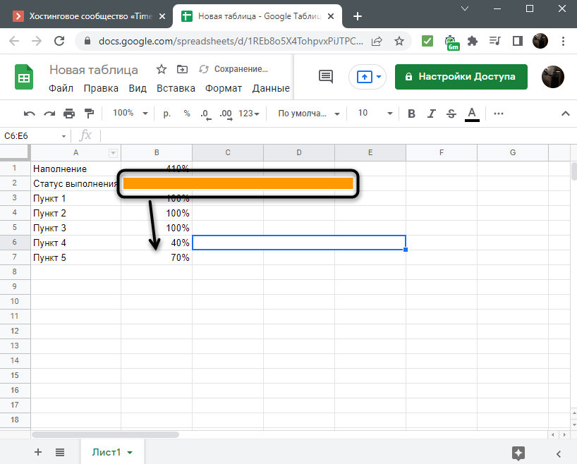
- Измените любое из значений на большее или меньшее и посмотрите, как изменяется длина графической шкалы.
Я перечислю все используемые в формуле =SPARKLINE(B1;<"charttype"\"bar";"max"\СЧЁТЗ(A3:A7)*100%>) параметры, чтобы у вас не возникло вопросов по содержимому. Кстати, саму формулу вы можете просто скопировать и вставить с заменой номеров ячеек.
- «charttype»\»bar» – тип используемой диаграммы, в данном случае это шкала.
- «max»\СЧЁТЗ(A3:A7)*100%> – максимально допустимое значение в наборе данных. Набором данных являются пункты с процентами.
- «color1″\»red» – отсутствует в данном представлении формулы, поскольку в шкале используется только один цвет для любого состояния. Понятно, что этот параметр отвечает за цвет шкалы, о его применении я расскажу далее.
Создание меняющегося цвета для графической шкалы
Простая одноцветная шкала для отображения процентов выполнения создается очень быстро и просто, в чем вы уже убедились. Немного сложнее будет ее модернизировать так, чтобы цвет менялся в зависимости от количества процентов. Для этого понадобится функция ЕСЛИ (она же IF), но сама формула по размеру будет большой.
- Для начала перед функцией диаграммы в ячейке объявите IF(, поставив только открывающуюся скобку.
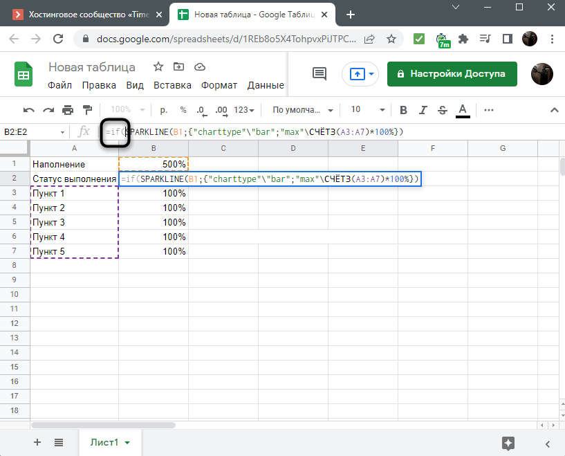
- После этого введите B1, где B1 – номер ячейки с общим подсчетом процентов. 250% вы можете заменить на любое значение.
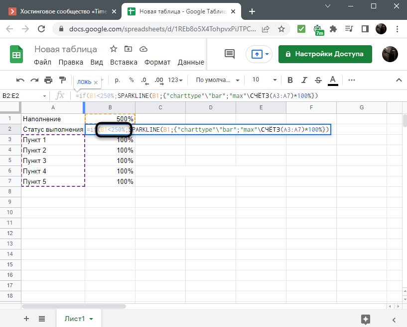
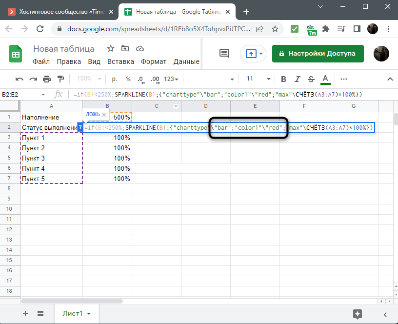
- Модернизируйте формулу, поставив после типа графика часть «color1″\»red», о которой уже шла речь выше. Цвет тоже замените на любой, но обязательно держите его в двойных кавычках.
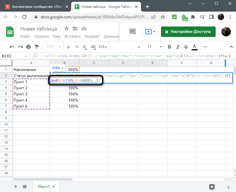
- Переместитесь в конец формулы, поставьте точку с запятой и пропишите IF(AND(B1>250%;B1<400%); для среднего значения.
- После этого вставьте ту же часть функции, начиная со SPARKLINE, но замените цвет уже на другой.
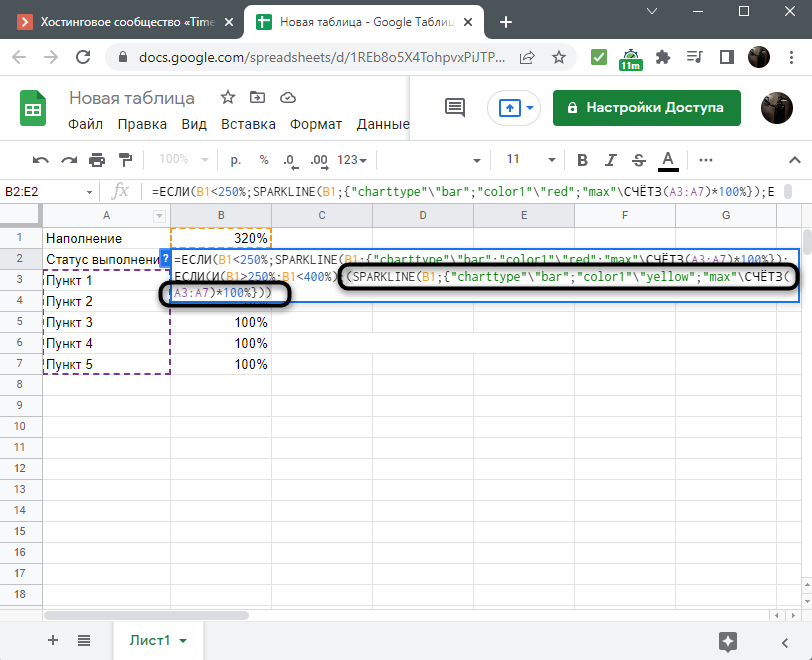
- Поставьте точку с запятой в конце, снова вставьте формулу графика и поставьте для него третий цвет. Этот вариант сработает в том случае, если значение не равняется ни одному из перечисленных выше условий.
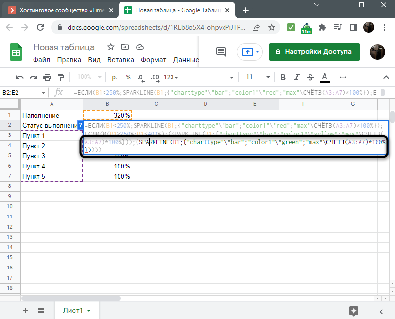
- Нажмите Enter для применения изменений и посмотрите, стал ли цвет графика другим.
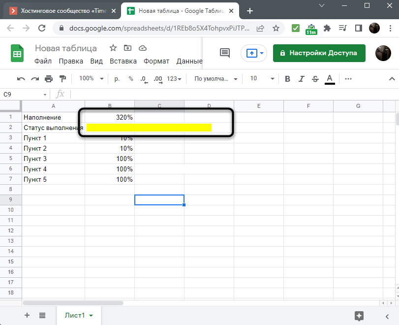
- Поменяйте проценты и продолжайте отслеживать изменения.
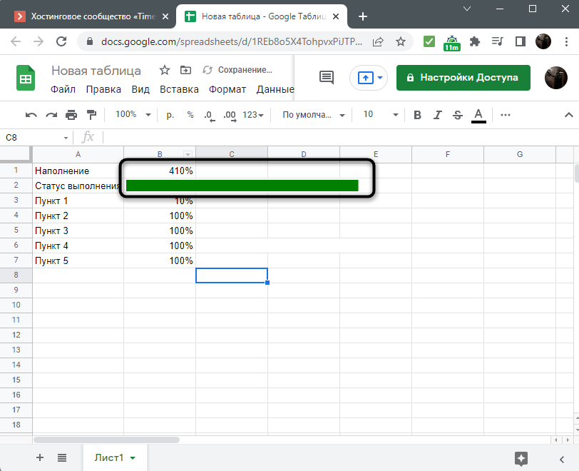
Может быть, объяснение кажется слишком сложным, но вам важно понять, какие ячейки участвуют в расчете, чтобы заменить их на свои в формуле. Саму формулу можно целиком скопировать и только поменять цвета с номерами ячеек. Специально для этого я оставляю проверенную версию ниже, которую и создавал в процессе написания данной статьи.
=ЕСЛИ(B1<250%;SPARKLINE(B1;<"charttype"\"bar";"color1"\"red";"max"\СЧЁТЗ(A3:A7)*100%>);ЕСЛИ(И(B1>250%;B1<400%);(SPARKLINE(B1;<"charttype"\"bar";"color1"\"yellow";"max"\СЧЁТЗ(A3:A7)*100%>));(SPARKLINE(B1;<"charttype"\"bar";"color1"\"green";"max"\СЧЁТЗ(A3:A7)*100%>))))
Да, понадобится потратить немного времени и разобраться с тем, как работает эта длинная сложная формула, однако результат того стоит, ведь всегда удобно видеть перед глазами шкалу выполнения задач, особенно когда она меняет свой цвет в зависимости от состояния. Впрочем, ничего не мешает оставить шкалу одноцветной и просто следить за ее размером относительно объединенных ячеек.
Google Sheets Percentage Formula (5+ Easy Examples)
Expressing quantities in percentages always helps give a better sense of proportion. It helps us visualize the quantity better in our heads and is great for making comparisons.
It’s no wonder that most common quantities like sales tax, discounts, bank interest rates, etc. are commonly expressed in percentages. In this tutorial, I will show you how to do percentages in Google Sheets using the Google Sheets percentage formula and other applications.
Table of Contents
What is a Percentage?
The term percent or percentage means one part of a hundred. It’s a fundamental concept for everyday life, and that’s one reason I wanted to cover it here. I use it to calculate tips at restaurants and to evaluate the effects of compounding interest on my mortgage. And it makes sense, right? I’m not going to express a ratio as a fraction of a random number. Instead, I’ll give it a base of 100. That’s the foundation of percentages.
You can also find the percent for a set of data. I’ll show you how to do that below. In that case, you’ll use the total data set as the denominator (instead of the base 100). It will give you a percent of your total, and you can format that as a percent in Google Sheets.
The Google Sheets Percentage Formula
How do you use the percentage formula in google sheets? You just use an equal sign, then divide one number over another. As you know, I usually break my spreadsheet formulas down into their corresponding syntax. I cover what you need to include in the parenthesis to get them to work. That’s not needed for the percentage formula in Google Sheets, because no formula looks like =PERCENT().
Instead, you’ll just use division over the full range of data. If you want to format it like a normal formula, it looks like this.
Here, X represents the portion of the whole and Y represents the whole. So 15% would be =15/100. Note that this formula gives you a fractional number, which you can then turn into a percent with formatting. And there’s a quick way to do that. I find it easiest to use the percentage button when formatting a percent in Google Sheets. But that’s not a formula.
Want a deeper dive? I’ll show my step-by-step instructions on how play with percentages below. I’ll include screenshots so you can follow along with each step of my process.
Why Use The Google Sheets Percentage Formula (s)?
The percentage format in Google Sheets is one of the most useful number formats. It helps you express values in percentages by not only adding a percentage sign next to it, but also by converting the number to a percentage value.
So if you have a fractional number like, say, 0.15 in a cell, formatting it with the percentage format automatically converts it into 15%.

All you need to do is select the cell, and click on the ‘%’ button from the Google Sheets toolbar. Here’s what it looks like on your toolbar.

Coming to the question of why we use percentage in Google Sheets, take a look at the images below. Notice that the Value Added Tax percent is formatted differently for each sheet. The VAT is displayed as a fraction of the first image, while the same value is displayed as a percentage in the second one.


I don’t know about you, but I find the second spreadsheet much easier to read than the first. And that’s why we use percentages in Google Sheets. Let’s move on to some more advanced ways to use this. Here are a few practical situations where I find this helpful:
- calculating the Percentage of proportion
- calculating the Percentage of the total
- calculating the Percentage change
There are several other situations in which the percentage can be applied, but I’m going to concentrate on these three in this tutorial.
How to Automatically Format as Percentage
Instead of using the percent toolbar to convert decimals to percentage, you can also turn the value into percentage directly. That’s done with the percent button. There’s also a formula you may want to try out. It’s supposed to automatically format as percentage.
To use it, add the TO_PERCENT function to your percentage formula in Google Sheets. For example, in our sheet above, I can automatically convert the value to a percentage using the formula:
=TO_PERCENT (C2/B2)

Note that the TO_PERCENT formula is currently the worst way to format a percentage in Google Sheets. It doesn’t automatically change your formatting into a percentage. Instead, it just completes your formula and puts your number into whatever format you’ve already chosen for the cell. That means you’ll have to click that “format as percent” button to get it to look right. For me, that makes this the worst way to calculate percentages in Google Sheets.
Here’s a video I made that shows how the TO_PERCENT formula works (when it actually does the automatic formatting).
How to Calculate Percentage Using *100
Another way I calculate percent in Google Sheets directly is by dividing the value of the total and multiplying it by 100 using the formula for percentage in Google Sheets below. It’s exactly what you’d do on paper to show a fraction as a percent. So, this should look familiar. Here’s the percent formatting formula:
(=(Value/total number)*100).
Using my example sheet above, we would use the formula =(C2/B2)*100

In this case, the number won’t show the percentage sign, but it has already been converted to a percentage by multiplying by 100. Note that using the percent button on this would show an incorrect result. So use this only if you’re looking to express percentages automatically and without the percent sign.
Example Spreadsheet
Want to follow along as I demonstrate how to calculate percentages? Please make a copy of my example spreadsheet. It contains my demonstrations on how to use the PERCENTIF function, divide COUNTIF functions over totals, and calculate the percentage of a proportion. If you learn like I do, you may find it faster to see my actual examples in the spreadsheet.
Note that all of my examples below come from this example spreadsheet. You can follow along in your own copy and make changes to see how it affects the results.
How to Calculate Percentage of a Proportion
The first application of percentages is in calculating the percentage of a proportion. In other words, what portion of a task belongs to or does not belong to a certain category?
For example, in the table below, we have the sales target allotted for each employee in Column B, and the sales made by them are given in Column C.

Let us say we want to calculate what percent of their allotted target each person has achieved. The general formula for this situation would be:
Sales Made / Allotted Target * 100
To apply this general formula to the above dataset, we need to follow the steps given below:
- Select cell D2 (where the first row’s result will be displayed).
- Type the formula =C2/B2

- Press the ‘Format as percent’ button (%) from the toolbar. Alternatively, you could navigate to Format->Number->Percent from the menu bar. This will convert the result of the formula to a percentage and display a ‘%’ sign next to the result.

- You should see the result in the second row of column D.
- Drag down the fill handle to copy the formula to the rest of the cells in column D.

- If you see the results include decimal places, you can choose to remove the decimal so you now have the percentage rounded up to the nearest whole number.

You now have a list of percentages of sales made by each employee. You will find it is easier to see who has been most efficient in achieving their targets.
How to Calculate the Percentage of Total
Next, let us look at a situation where we have the sales made by each employee (assuming that they all have a combined target).

We want to know what percentage of the total sales each employee has made.
The general formula for a given employee would be:
Sales made by the employee / Total sales * 100
The total sales made by all employees can be calculated using the SUM function as follows:
=SUM(B2:B6)
To apply this general formula to the above dataset, we need to follow the steps given below:
- First, calculate the total sales made. For this, we can use the SUM function and display the result in cell B7. The formula for the total will be =SUM(B2:B6).

- Next, select cell C2 (where the first row’s result will be displayed).
- Type the formula =B2 / $B$7

- Press the ‘Format as per cent’ button (%) from the toolbar. Alternatively, you could navigate to Format->Number->Percent from the menu bar. This will convert the result of the formula to percentage and display a ‘%’ sign next to the result.
- You should see the result in the second row of column C.

- Drag down the fill handle to copy the formula to the rest of the cells in column C.

- If you see the results include decimal places, you can choose to remove the decimal so you now have the percentage rounded up to the nearest whole number.

You now have a list of percentages of total sales made by each employee.
You will find it is easier to see which employee contributed the most or least to the total sales. You can even use this to gauge their performance over a period of time.
We will also take a look at a situation like this in the next section.
Explanation of the Formula
You will notice that we used more or less the same basic formula as the previous case, but with a very slight difference. We used an absolute reference to the total sales made (cell B7).
The dollar sign ($) is used to specify that a reference is absolute, so it does not change when you copy the formula to the other cells.
We do this to ensure that every cell value of column B gets divided by the same cell value (in B7). Thus, every new result in column C will get calculated based on the sum in cell B7:
=B2/$B$7
Note: If we sum up all the percentages in column C, we should get a total of 100%, which obviously makes sense.

How to Calculate Percentage Change
Once you have the percentage of sales of an employee calculated for every month or week, it then becomes easy to monitor their performance.
You can easily see if their percentage increases or decreases.
Let us now take a situation where we have the sales made by employees in week 1 and in week 2.

We want to know what percentage change (improvement or decline) there has been in each employee’s sales.
The general formula for this situation would be:
(New Value - Old value) / Old value * 100
To apply this general formula to the above dataset, we need to follow the steps given below:
- Select cell D2 (where the first row’s result will be displayed).
- Type the formula =(C2-B2)/B2

- Press the ‘Format as per cent’ button (%) from the toolbar. Alternatively, you could navigate to Format->Number->Percent from the menu bar. This will convert the result of the formula to percentage and display a % sign next to the result.
- You should see the result in the second row of column D.

- Drag down the fill handle to copy the formula to the rest of the cells in column D.

- If you see the results include decimal places, you can choose to remove the decimal so you now have the percentage rounded up to the nearest whole number.

You now have a list of percentage increases/decreases in each employee’s sales over a one-week period.
You will find it is easier to see, analyze, compare, and trace their performances over the course of a few weeks, months, or even years.
How to Calculate Percentage Based on Criteria
There are more applications of the percentage calculator in Google Sheets. One of them is calculating percentages based on criteria. To do this with we will need to combine the PERCENT function with the IF function.
The PERCENTIF syntax is as follows:
=PERCENTIF( Range, Criterion)
Range: This is the data set that is to be converted to a percentage.
Criterion: This is the argument used to filter out data from the range. It can be a cell reference or a value in quotation marks. It can also include logical expressions like greater than(>) and less than(<).
Let’s look at our example below:

We can get the percentage of the sales that are less than 10,000 using the formula:
=PERCENTIF(C2:C9, ">10000")
How to Calculate a Percentage of Checkboxes in Google Sheets
It is also possible to get the percentage of checkboxes ticked or unchecked in Google Sheets. The process is a bit more mathematical than most functions since you will need a formula that will count the number of checked boxes.
In this case, we will use the COUNT formula, which will give us the number of checkboxes that are either ticked or unchecked. We can then divide this by the number of total checkboxes and then convert it to a percentage.
The basic Google Sheet formula for percentage is:
=COUNTIF(range,True) / COUNTA(range)
Let’s look at our example spreadsheet below:

We can get the percentage of employees paid by getting the number of checkboxes divided by the total number of checkboxes.
We will use the formula:
=COUNTIF(C2:C6,True) / COUNTA(C2:C6)

We can then convert the decimal into a percentage by clicking the % icon on the quick access toolbar. This will give us 40%.
Increase and Decrease Numbers by a Percentage
Here’s how you increase or decrease numbers by a percentage in Google Sheets. It’s a pretty simple process, and I’ve got an example built into my example spreadsheet. Here’s what my sheet looks like before I apply the formula. Next, we’ll talk about how to increase by a percentage.

Increase by Percentage
To increase a value by a percentage, we can use the formula:
=Amount*(1+%)
This formula multiplies the value by the percentage increase to give you the results. In our example, we would use the formula:
=A2*(1+B2)

This gives us 1200 as the result.
Decrease by Percentage
The way to decrease a value by a percentage is similar to increasing it. The only difference is that we will use a minus instead of a plus in the formula.
=Amount*(1-%)
In our example, we would use the formula:
=A5*(1-B5)

This will give us 900 as the result. The formula in the brackets is used to get the percentage that we will multiply the value with, for example, (1+20%) will give us 120%, and (1-10%) will give us 90%.
Conclusion
In this tutorial, I showed you the Google Sheets percentage formula options. Of course, there are a host of other situations where percentages would need to be calculated, but I assume these three examples would be enough to give you a basic idea of the possibilities you have, thanks to the ‘Format as percent’ feature.
I encourage you to apply this small convenience to your daily data processing needs and hope it helps you get your work done at least a small percent quicker. You can also check out our guide to the percentile function in Google Sheets. I made a whole video about how to use it.
Other Google Sheets tutorials you may like:
-
- How to Calculate Weighted Average in Google Sheets
- How to Calculate the Standard Deviation in Google Sheets
- How to Divide in Google Sheets
- How to Multiply in Google Sheets
- How to Subtract in Google Sheets
- Convert Decimal to Fractions in Google Sheets
Как узнать сумму из периода с условиями в Google Таблице

При взаимодействии с Гугл Таблицей пользователь может создавать записи каждый день, указывая дату и какое-нибудь число рядом с ней, к примеру сумму заработанных денег. Здесь может быть еще одно условие – вид деятельности, в котором эта сумма была заработана. Пройдут недели или даже месяцы, таблица наполнится и понадобится узнать, сколько денег было заработано за определенный период в определенной сфере. Вычислить необходимую сумму можно двумя разными методами, которые я и хочу наглядно продемонстрировать.
Обращу ваше внимание на то, что во вступительном абзаце я описал только пример. Практических методов использования описываемых ниже формул может быть безграничное количество. Все зависит исключительно от ваших целей и исходных данных. Это же относится и количеству условий, ведь все формулы можно масштабировать, что тоже будет продемонстрировано, но в конце статьи, чтобы не усложнять и без того не самое простое объяснение.
Исходные данные и подготовительные работы
Я возьму таблицу, содержимое которой уже описал вкратце выше, вместе с этим проведу некоторые подготовительные работы, чтобы оптимизировать ее и облегчить вычисления в дальнейшем. Вы можете полностью скопировать этот пример или использовать его только для ознакомления с принципом работы формул. Давайте начнем с перечисления исходных данных:
- В одном столбце у нас есть последовательные дни, которые и будут являться периодом в будущем.
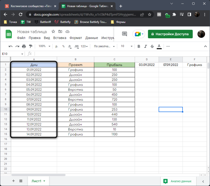
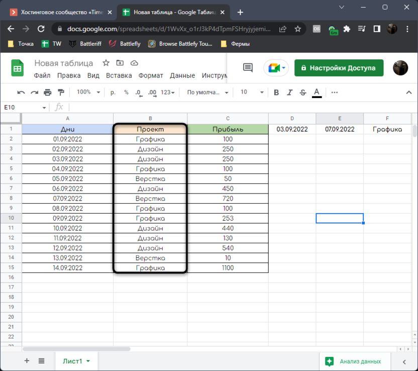
- Следующий столбец показывает сферу деятельности, которой пользователь занимался в каждый из этих дней.
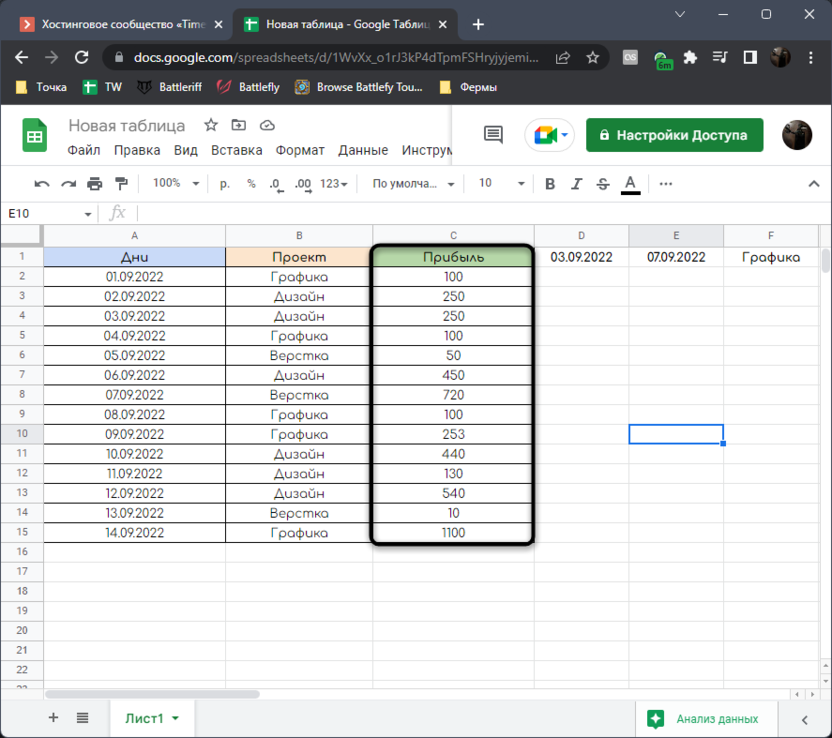
- Последний – полученная прибыль, сумму которой и будем считать в зависимости от выставленного периода и дополнительных условий.
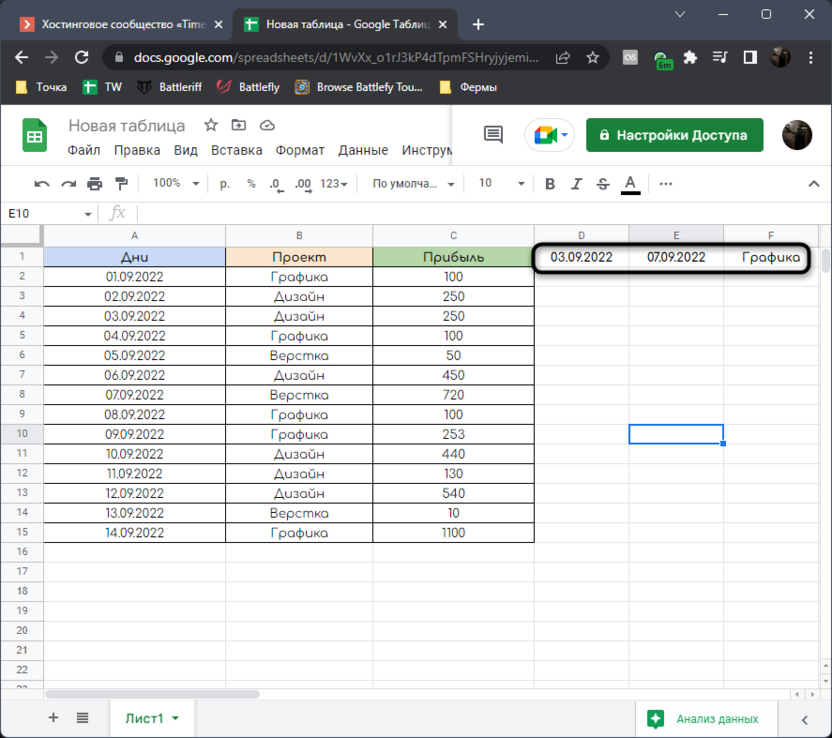
- В строках выше я указываю начальную дату периода, конечное число и сферу деятельности, заработок из которой нужно узнать.
Вы можете использовать просто численные обозначения дней от одного до бесконечности, другой формат даты, добавить несколько условий или суммировать не прибыль, а другие значения. Все зависит исключительно от имеющейся у вас на руках таблицы.
Теперь быстро затронем простую тему подготовительных работ. Я буду использовать проверку данных, чтобы сформировать список в этих самых вспомогательных ячейках. Это поможет не редактировать их каждый раз при изменении периода или условий, а просто выбирать подходящее значение из списка.
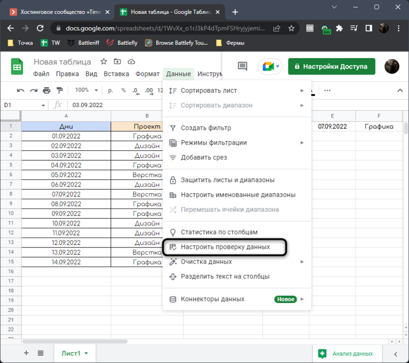
- Для начала разберемся с начальной датой периода. Выделим эту самую ячейку и развернем меню «Данные».
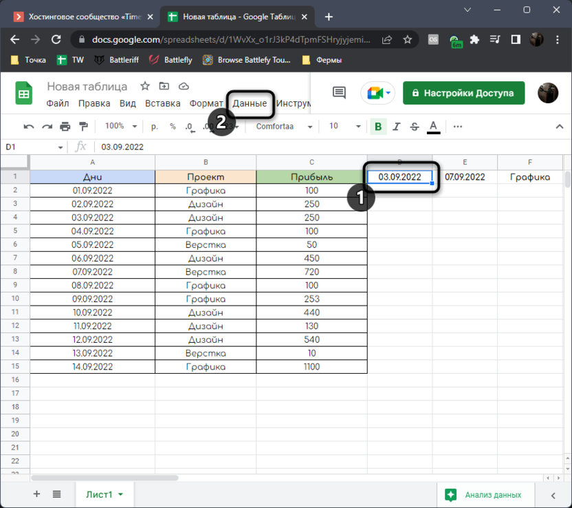
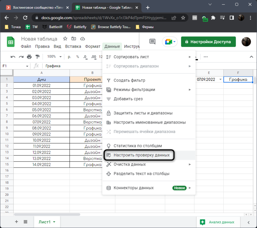
- Из него выберите пункт «Настроить проверку данных».
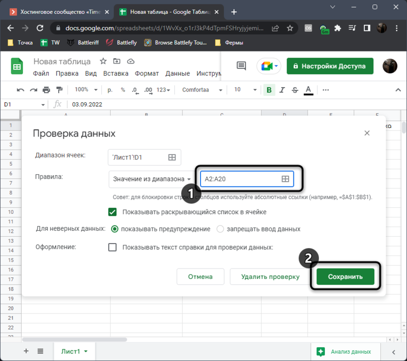
- Понадобится ввести только одно изменение – указать столбец, из которого эти данные будут браться. Соответственно, выделите диапазон, где записаны все ваши числа, после чего сохраните изменения.
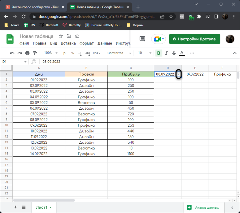
- Теперь рядом с числом появится кнопка со стрелкой вниз.
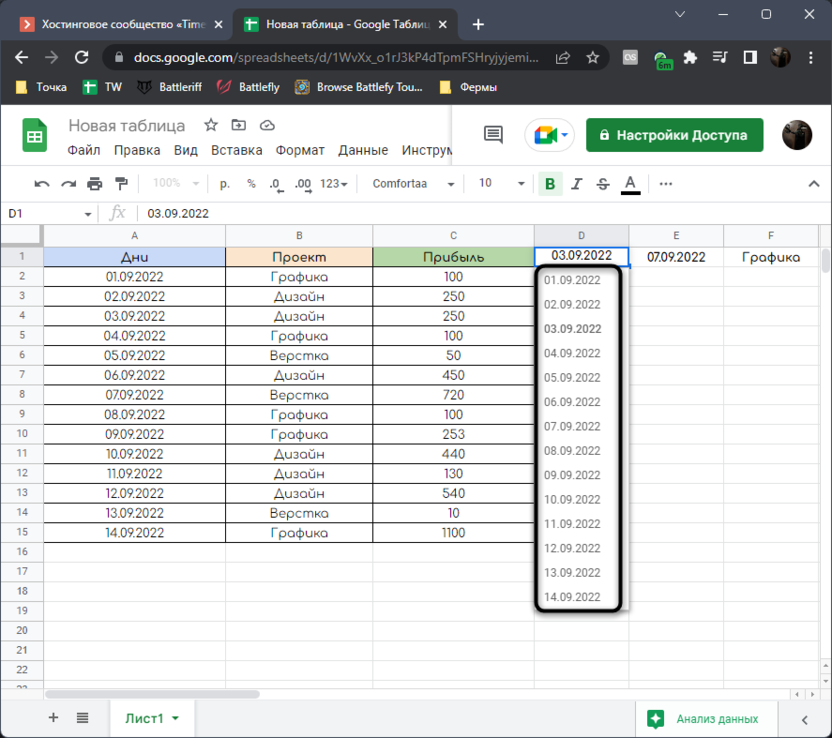
- Нажмите ее для отображения списка всех дат. Из него можете выбрать любую, которая и будет обозначать начало вашего периода.
- Абсолютно то же самое проверните и с ячейкой конечной даты, чтобы точно так же переключаться при необходимости.
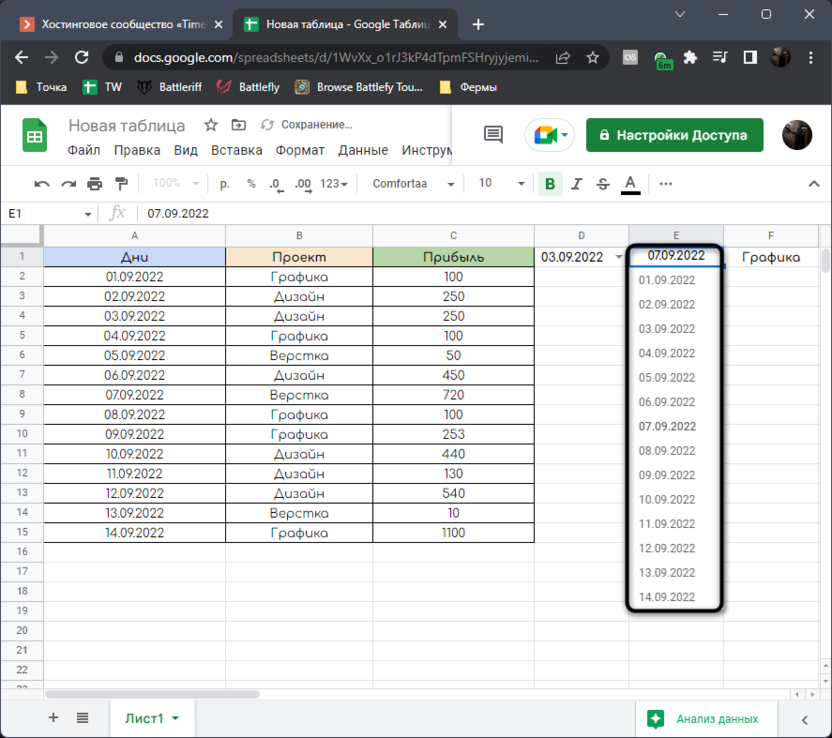
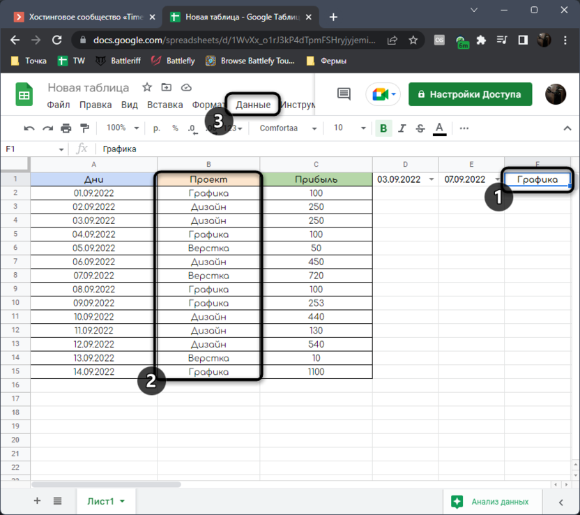
- С дополнительными условиями все примерно так же. Выделите пустую ячейку, где хотите сформировать список, запомните номер столбца и переходите в меню «Данные».
- Снова вызовите функцию «Настроить проверку данных» и в новом окне задайте подходящий диапазон точно так же, как делали это ранее.
- Главное — записывайте одинаковые сферы деятельности одинаковыми символами, чтобы список формировался правильно, без лишних дублей.
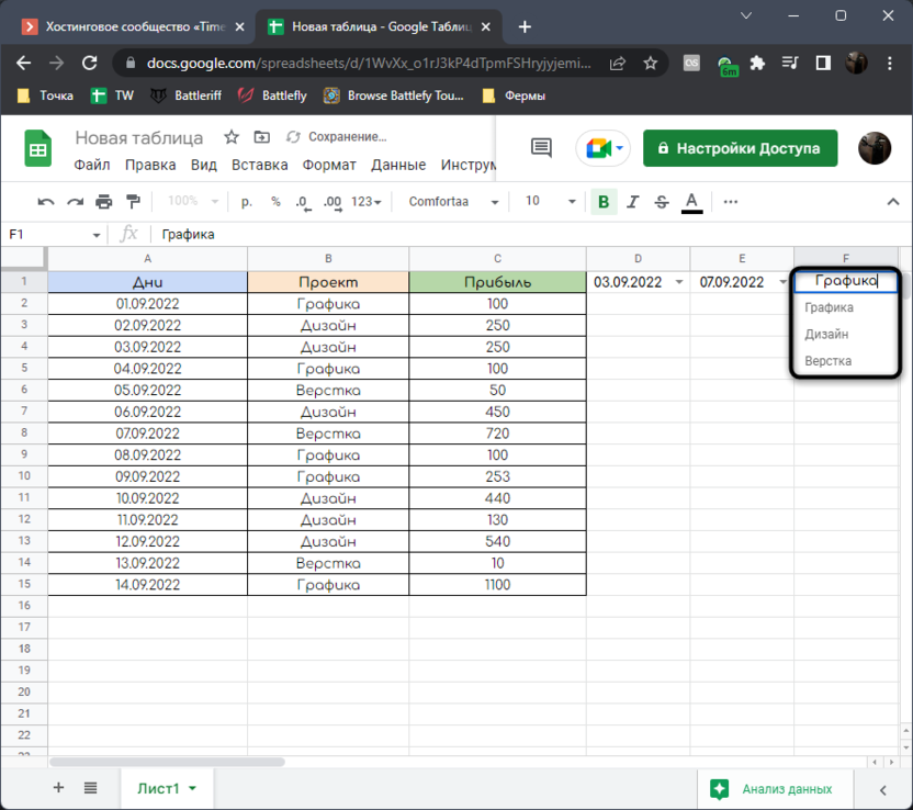
На этом ознакомление с самой таблицей и проведение подготовительных работ завершено, поэтому давайте перейдем к разбору первой, более сложной формулы вычисления необходимой нам информации.
Комьюнити теперь в Телеграм
Подпишитесь и будьте в курсе последних IT-новостейСпособ 1: Использование функции AND и СУММЕСЛИ
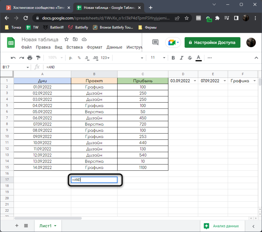
Функция AND в Google Таблицах позволяет сравнить неравенство и вывести в ячейку значение ИСТИНА или ЛОЖЬ, отталкиваясь от того, подходит ли условие неравенства. Благодаря этой функции мы создадим вспомогательный столбец, при помощи которого будем вычислять все дни, входящие в необходимый нам период. Давайте наглядно разберем все составляющие первой формулы, которая будет нужна для дальнейших расчетов.
- Выделите первую ячейку в том столбце, который можете сделать вспомогательным. Объявите в нем функцию =AND.
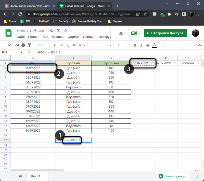
- Далее разверните скобки и укажите первое условие неравенства (A2>=$D$1;). Обратите внимание на то, что ячейка D1 является статичной благодаря добавлению константы, то есть не будет растягиваться при дальнейшем формировании столбца.
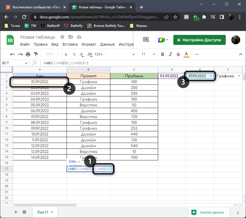
- Второе условие A2, где E1 – ячейка с последней датой периода.
- Нажмите Enter для подтверждения формулы и растяните ее ровно на столько клеток вниз, сколько у вас ячеек в столбце с датами. В итоге она будет иметь примерно такой вид: =AND(A2>=$D$1;A2<=$E$1;B2=$F$1).
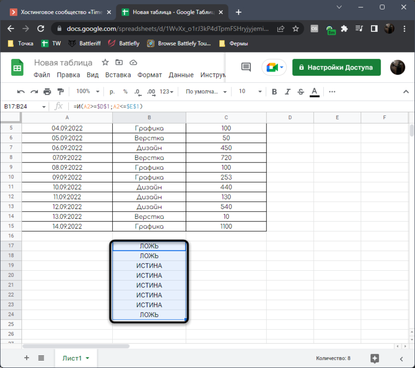
При помощи этой функции мы вычисляем даты, которые актуальны для выбранного пользователем периода. Значения ИСТИНА или ЛОЖЬ будут меняться в зависимости от того, какие даты вы будете самостоятельно указывать в качестве начала и конца периода. Соответственно, если значение ИСТИНА, значит, дата входит в период и значение прибыли будет включено в формулу. Если ЛОЖЬ, ячейка пропускается и осуществляется переход к следующей.
С первой частью формулы закончили, остается только создать основные расчеты, в которые и будут включены значения ИСТИНЫ и ЛЖИ из вспомогательного столбца. В этом нам поможет СУММЕСЛИ. Эта функция считает значение только в том случае, если ее устраивает заданное условие. Запись этой формулы в нашем случае выглядит следующим образом:
- Объявите функцию =СУММЕСЛИ в том месте, где хотите разместить сам результат суммирования прибыли или других данных, вычисляемых в периоде.
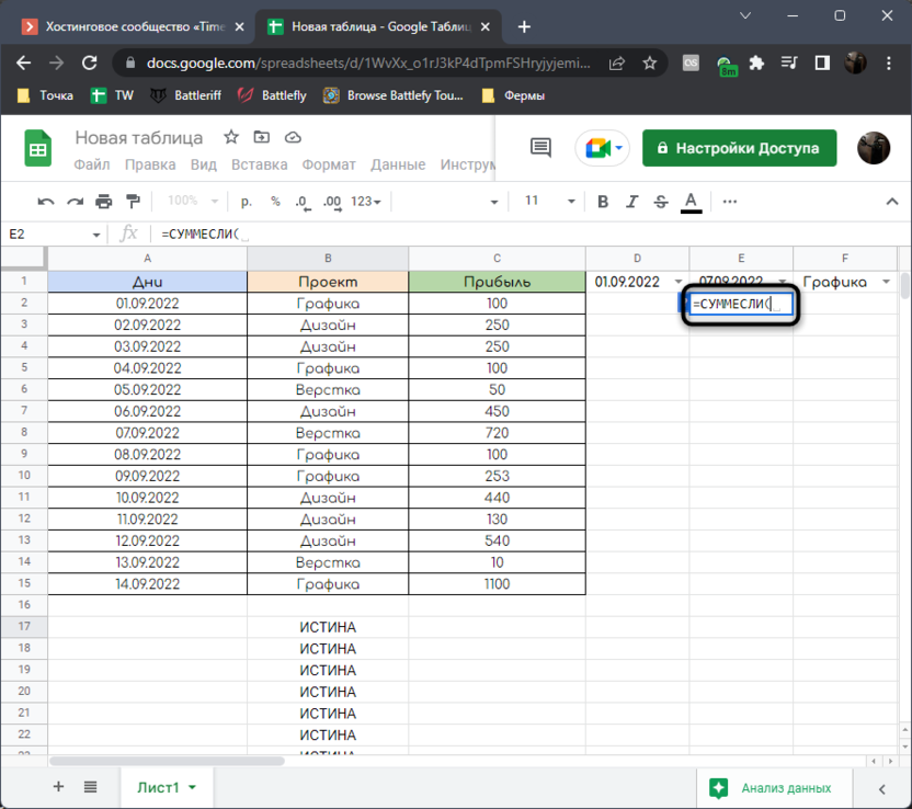
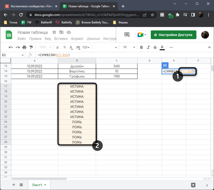
- В качестве первого столбца для проверки укажите все ячейки с ИСТИНА и ЛОЖЬ, которые мы формировали ранее.
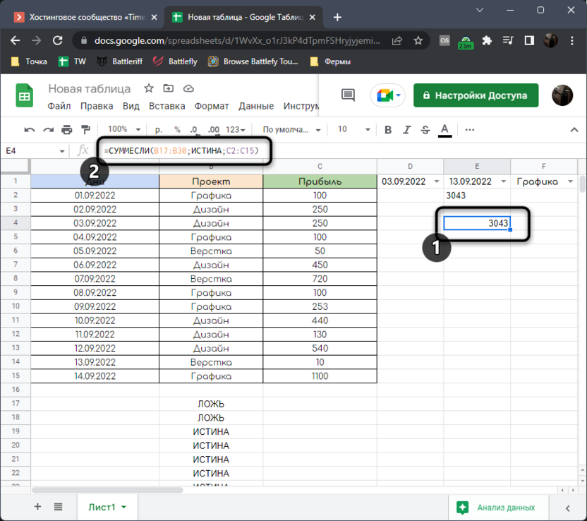
- Поставьте точку с запятой, добавьте ИСТИНА, поставьте еще раз точку с запятой и укажите диапазон данных со значениями, сумму которых нужно рассчитать. Нажмите Enter и посмотрите на результат.
- Я вручную выделяю все ячейки, которые входят в период по дням и смотрю, что формула работает корректно.
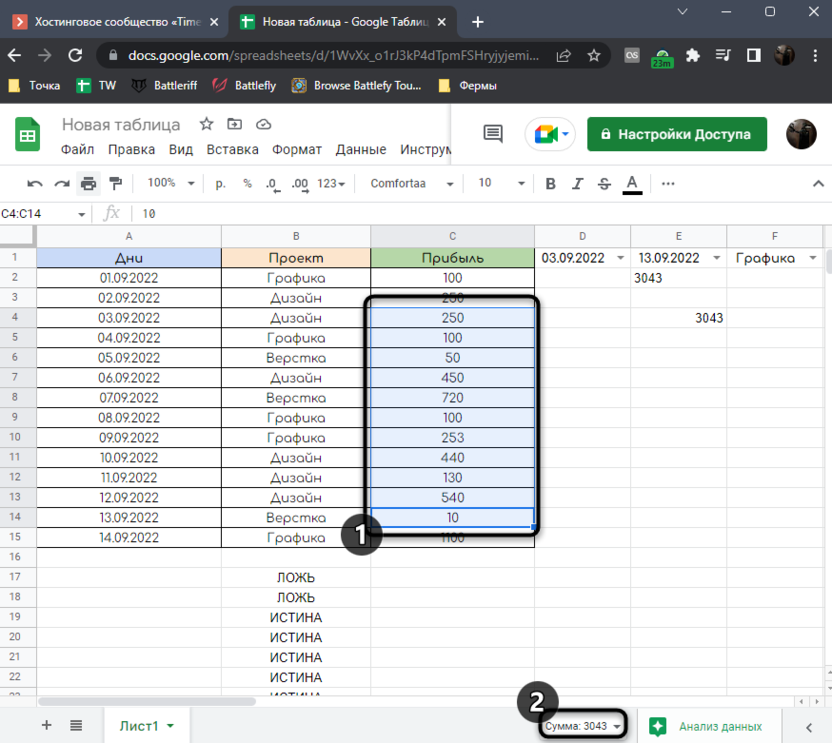
Давайте более наглядно разберем ее. Формула имеет вид =СУММЕСЛИ(B17:B30;ИСТИНА;C2:C15). В первую очередь указывается проверяемый диапазон, далее – условие, которое нас устраивает, то есть это должна быть ИСТИНА. Последний аргумент – данные, которые будут суммироваться, если равно ИСТИНА, то есть столбец с нашей прибылью.
Способ 2: Использование функции SUMPRODUCT
Предыдущий метод имеет один весомый недостаток – необходимость использования вспомогательного столбца и совмещение нескольких функций. Да, этот столбец можно скрыть или переместить на другой лист, но это не всегда уместно. Если и вам кажется, что первый метод не очень подходит, давайте разберемся с тем, как выполнить эту же задачу, но с использованием функции SUMPRODUCT.
Объяснить само действие функции немного сложнее. Мы задаем для нее несколько аргументов с логическими условиями, после чего указываем, что нужно суммировать только те значения, которые подпадают под заданные условия. В наглядном виде, если речь идет о решении сегодняшней задачи, использование этой функции выглядит так:
- Сначала объявите =SUMPRODUCT или =СУММПРОИЗВ на русском языке, в любой удобной клетке, куда хотите вывести результат.
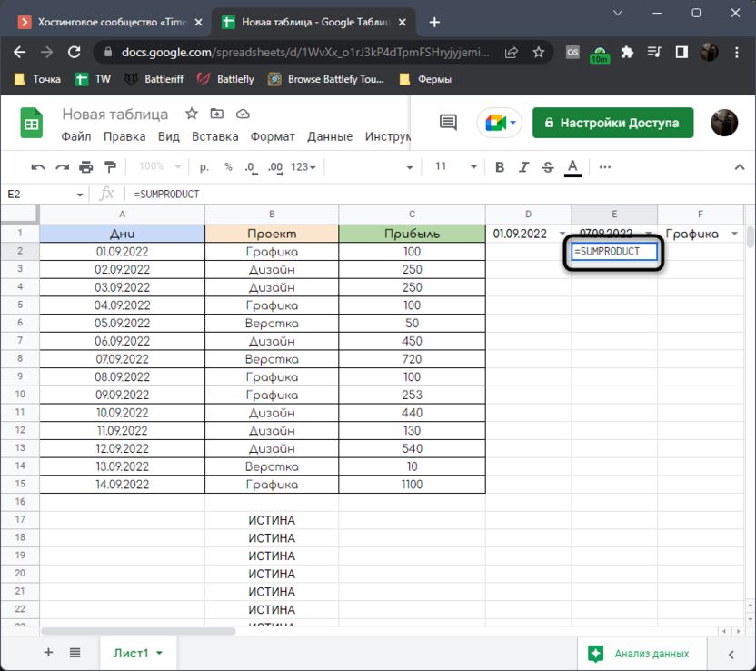
- Откройте кавычки и укажите, что диапазон числа из диапазона дат должен быть больше или равняться первому числу в периоде. Это делается точно так же, как и при создании вспомогательного столбца в Способе 1.
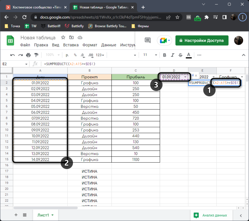
- Закройте скобки после первого условия и поставьте знак *, то есть в нашем случае мы объединим предыдущее условие со следующим. Как раз откройте скобки и напишите второе условие, указав, что значения в диапазоне дат должны быть меньше или равняться последнему числу в периоде.
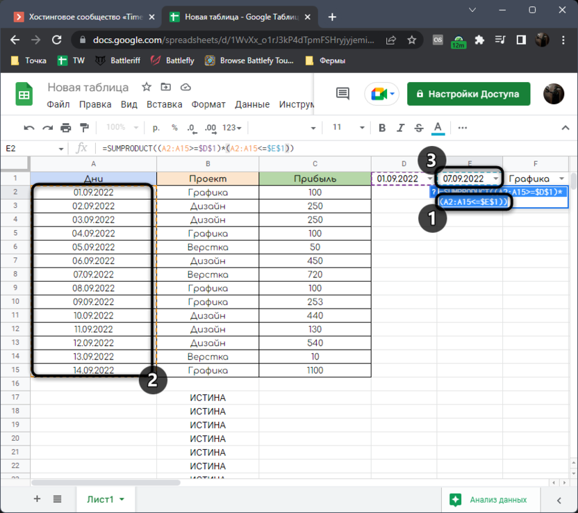
- Остается только добавить еще один знак * и дописать, что при истинных значениях условий нужно суммировать числа из диапазона с прибылью.
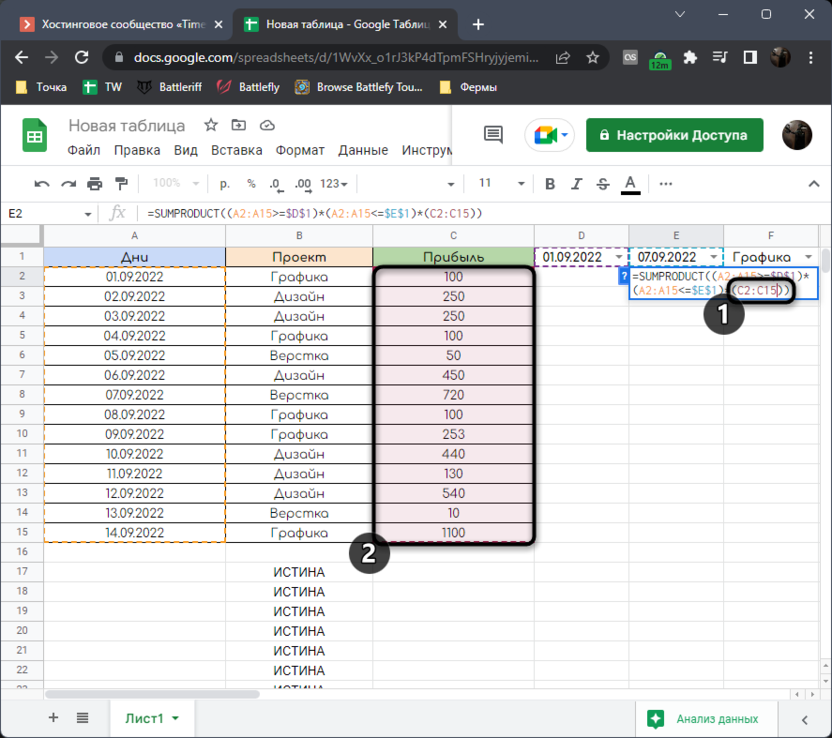
- Нажмите Enter и проверьте, сработала ли функция. Если нет, перечитайте мою инструкцию еще раз и проанализируйте ее составляющие со своими.
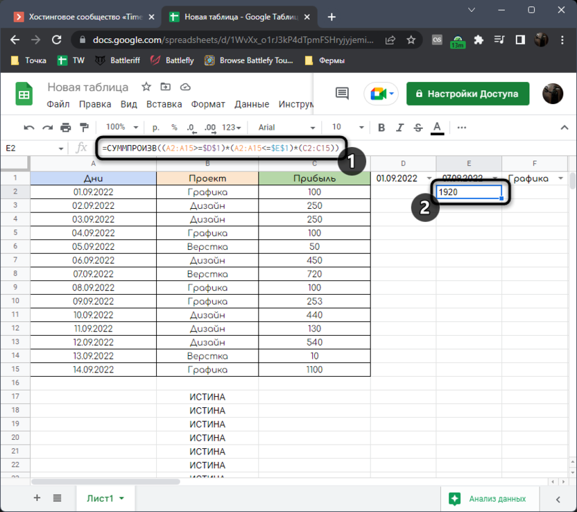
Полностью строка с этой формулой выглядит как =СУММПРОИЗВ((A2:A15>=$D$1)*(A2:A15<=$E$1)*(C2:C15)), поэтому можете просто скопировать ее и вставить, если номера ячеек в столбцах совпадают. В этой строке мы объявили два логических условия, после чего сказали формуле, какие данные стоит суммировать, если они устраивают заданные параметры.
Добавление условий к периоду
Как я и сказал, в конце разберем масштабирование наших формул, добавляя к ним различные условия. В моем случае это вид деятельности, которым человек занимался каждый день и получал за это прибыль.
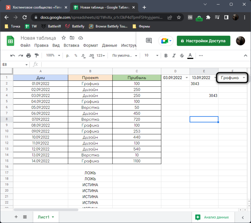
Получается, что при помощи описанных выше формул нужно посчитать сумму не только в заданном диапазоне, но беря в расчет еще и вид деятельности, записанный в столбце рядом. Каждую из формул придется немного модернизировать, поэтому начнем с первой.
- Активируйте первую ячейку из вспомогательного столбца с функцией AND и добавьте к ней еще одно условие, которое выглядит как B2=$F$1. B2 – первая ячейка с видом деятельности, а F1 – то самое условие, которое мы выбираем при расчетах. Его нужно закрепить, чтобы далее ячейка не съехала.
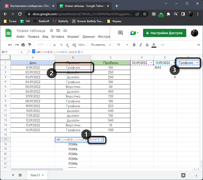
- Саму формулу растяните до последней ячейки вспомогательного столбца, зажав ее левой кнопкой мыши за правый нижний угол.
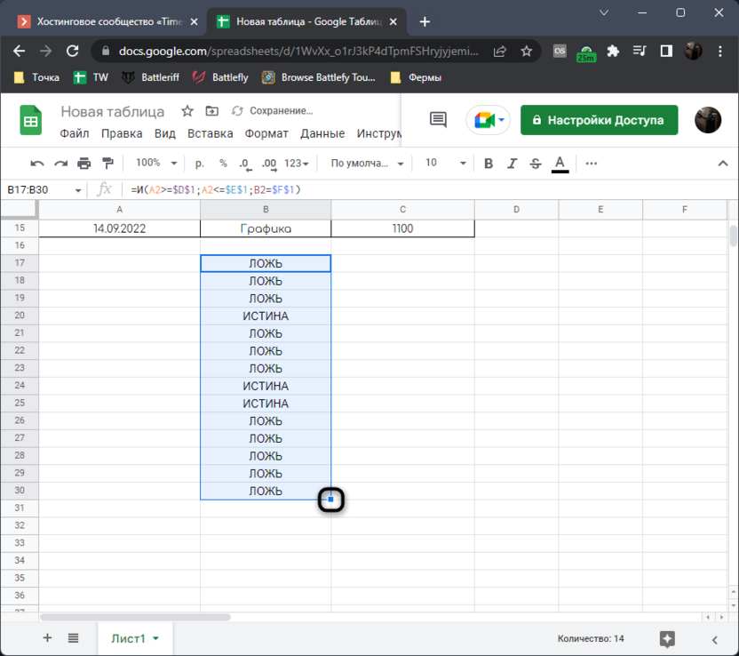
- В функции =СУММЕСЛИ изменения произойдут автоматически, поскольку она берет данные из ИСТИНА и ЛОЖЬ. Теперь вы видите, что формула считает по-новому, с учетом введенного условия. Таких условий может быть практически неограниченное количество.
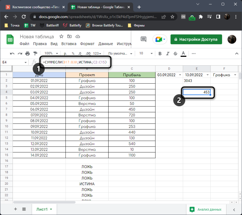
Если вам нужно, оставляю модернизированную функцию с добавлением одного условия.
=AND(A2>=$D$1;A2<=$E$1;B2=$F$1)
Примерно то же самое осуществляется и с формулой SUMPRODUCT, в которую после двух логических условий нужно добавить третье, выбирая весь диапазон с нашими условиями.
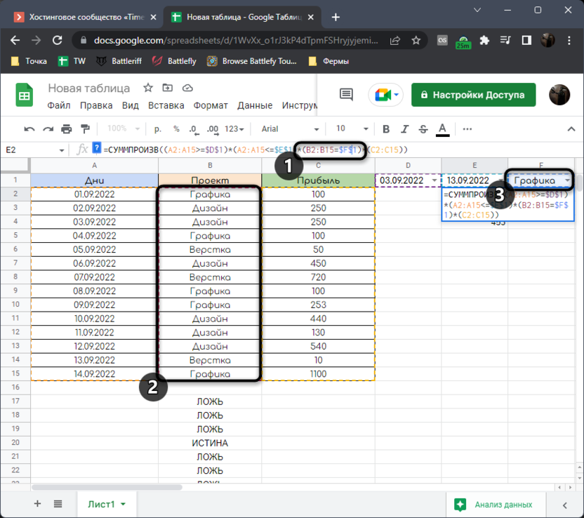
Результат получается точно такой же. Поначалу можно запутаться в такой длинной строчке, но если посмотреть выделенные столбцы и правильно определить последовательность действий, все становится предельно понятно.
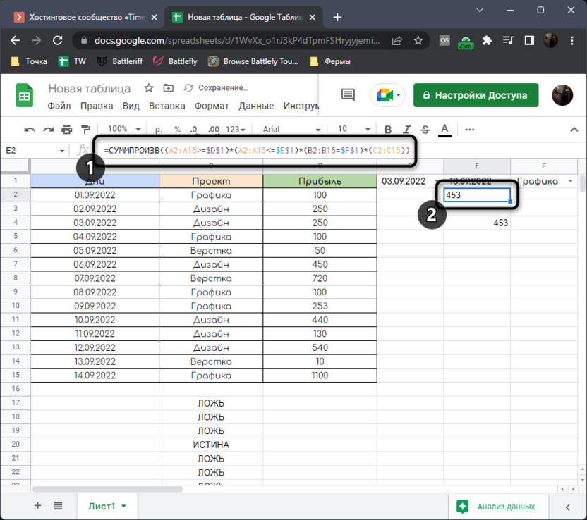
Как и в случае с предыдущей формулой, предоставляю модернизированный вариант, если вдруг решите его скопировать для дальнейшего использования.
=СУММПРОИЗВ((A2:A15>=$D$1)*(A2:A15<=$E$1)*(B2:B15=$F$1)*(C2:C15))
Мы с вами разобрались с выполнением не самой простой задачи. Вы узнали, что можете динамически изменять сам период для вычислений и добавлять различные условия. Если нужно, комбинируйте полученные результаты с другими формулами, создавайте сводные таблицы и многое другое. Если у вас возникнут вопросы по теме, смело задавайте их в комментариях, а я постараюсь предоставить оперативный ответ.